Blockwise coregistration

Often, biases are spatially variable, and a “global” shift may not be enough to coregister a DEM properly. In the Nuth and Kääb coregistration example, we saw that the method improved the alignment significantly, but there were still possibly nonlinear artefacts in the result. Clearly, nonlinear coregistration approaches are needed. One solution is xdem.coreg.BlockwiseCoreg, a helper to run any Coreg class over an arbitrarily small grid, and then “puppet warp” the DEM to fit the reference best.

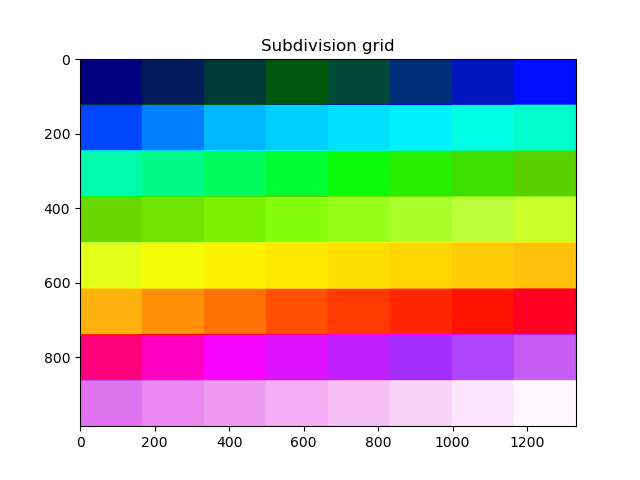
The BlockwiseCoreg class runs in five steps:

1. Generate a subdivision grid to divide the DEM in N blocks.

2. Run the requested coregistration approach in each block.

3. Extract each result as a source and destination X/Y/Z point.

4. Interpolate the X/Y/Z point-shifts into three shift-rasters.

5. Warp the DEM to apply the X/Y/Z shifts.

import geoutils as gu

import matplotlib.pyplot as plt
import numpy as np
from geoutils.raster.distributed_computing import MultiprocConfig

import xdem

We open example files.

reference_dem = xdem.DEM(xdem.examples.get_path("longyearbyen_ref_dem"))
dem_to_be_aligned = xdem.DEM(xdem.examples.get_path("longyearbyen_tba_dem"))
glacier_outlines = gu.Vector(xdem.examples.get_path("longyearbyen_glacier_outlines"))

# Create a stable ground mask (not glacierized) to mark "inlier data"
inlier_mask = ~glacier_outlines.create_mask(reference_dem)

plt_extent = [
    reference_dem.bounds.left,
    reference_dem.bounds.right,
    reference_dem.bounds.bottom,
    reference_dem.bounds.top,
]

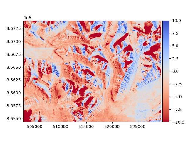
The DEM to be aligned (a 1990 photogrammetry-derived DEM) has some vertical and horizontal biases that we want to avoid, as well as possible nonlinear distortions. The product is a mosaic of multiple DEMs, so “seams” may exist in the data. These can be visualized by plotting a change map:

diff_before = reference_dem - dem_to_be_aligned

diff_before.plot(cmap="RdYlBu", vmin=-10, vmax=10)
plt.show()

Horizontal and vertical shifts can be estimated using xdem.coreg.NuthKaab. Let’s prepare a coregistration class with a tiling configuration BlockwiseCoreg is also available without mp_config but with parent_path parameters

# Create a configuration without multiprocessing cluster (tasks will be processed sequentially)
mp_config = MultiprocConfig(chunk_size=500, outfile="aligned_dem.tif", cluster=None)
blockwise = xdem.coreg.BlockwiseCoreg(xdem.coreg.NuthKaab(), mp_config=mp_config)

Coregistration is performed with the .fit() method.

blockwise.fit(reference_dem, dem_to_be_aligned, inlier_mask)
blockwise.apply()

aligned_dem = xdem.DEM("aligned_dem.tif")

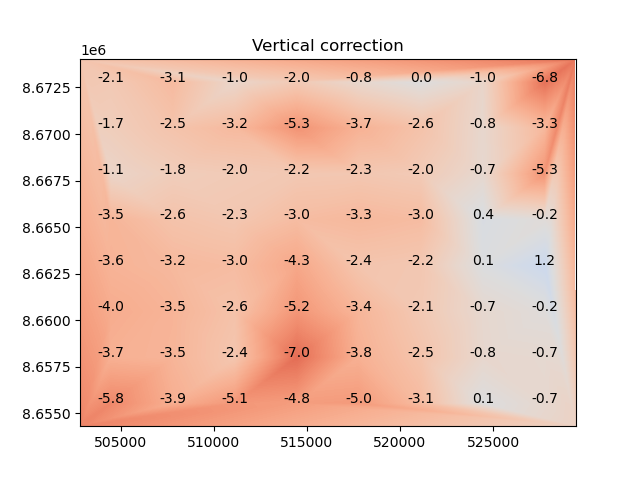
The estimated shifts can be visualized by applying the coregistration to a completely flat surface. This shows the estimated shifts that would be applied in elevation; additional horizontal shifts will also be applied if the method supports it.

rows, cols, _ = blockwise.shape_tiling_grid

matrix_x = np.full((rows, cols), np.nan)
matrix_y = np.full((rows, cols), np.nan)
matrix_z = np.full((rows, cols), np.nan)

for key, value in blockwise.meta["outputs"].items():
    row, col = map(int, key.split("_"))
    matrix_x[row, col] = value["shift_x"]
    matrix_y[row, col] = value["shift_y"]
    matrix_z[row, col] = value["shift_z"]


def plot_heatmap(matrix, title, cmap, ax):
    im = ax.imshow(matrix, cmap=cmap)
    for (i, j), val in np.ndenumerate(matrix):
        ax.text(j, i, f"{val:.2f}", ha="center", va="center", color="black")
    ax.set_title(title)
    ax.set_xticks(np.arange(cols))
    ax.set_yticks(np.arange(rows))
    ax.invert_yaxis()
    plt.colorbar(im, ax=ax)


fig, axes = plt.subplots(1, 3, figsize=(18, 6))
plot_heatmap(matrix_x, "shifts in X", "Reds", axes[0])
plot_heatmap(matrix_y, "shifts in Y", "Greens", axes[1])
plot_heatmap(matrix_z, "shifts in Z", "Blues", axes[2])

plt.tight_layout()
plt.show()

Then, the new difference can be plotted to validate that it improved.

diff_after = reference_dem - aligned_dem

diff_after.plot(cmap="RdYlBu", vmin=-10, vmax=10)
plt.show()

We can compare the NMAD to validate numerically that there was an improvement:

print(f"Error before: {gu.stats.nmad(diff_before[inlier_mask]):.2f} m")
print(f"Error after: {gu.stats.nmad(diff_after[inlier_mask]):.2f} m")

Error before: 3.42 m
Error after: 2.20 m