Note
Go to the end to download the full example code.
Slope and aspect methods#
Calculating terrain attributes—not only slope and aspect but also curvatures—requires estimating the elevation derivatives of the surface. xDEM offers three different ways to calculate elevation derivatives, which can result in slightly different results.
Here is an example of how to generate the two with each method, and understand their differences.
See also the Terrain attributes feature page.
References: Horn (1981), Zevenbergen and Thorne (1987), Florinsky (2009).
import matplotlib.pyplot as plt
import numpy as np

import xdem
We open example data.
dem = xdem.DEM(xdem.examples.get_path("longyearbyen_ref_dem"))


def plot_attribute(attribute, cmap, label=None, vlim=None):

    if vlim is not None:
        if isinstance(vlim, (int, np.integer, float, np.floating)):
            vlims = {"vmin": -vlim, "vmax": vlim}
        elif len(vlim) == 2:
            vlims = {"vmin": vlim[0], "vmax": vlim[1]}
    else:
        vlims = {}

    attribute.plot(cmap=cmap, cbar_title=label, **vlims)

    plt.xticks([])
    plt.yticks([])
    plt.tight_layout()

    plt.show()
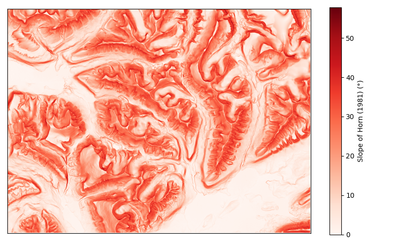
Slope with method of Horn (1981).
Note
(GDAL default), based on a refined approximation of the gradient (page 18, bottom left, and pages 20-21).
slope_horn = xdem.terrain.slope(dem, surface_fit="Horn")

plot_attribute(slope_horn, "Reds", "Slope of Horn (1981) (°)")
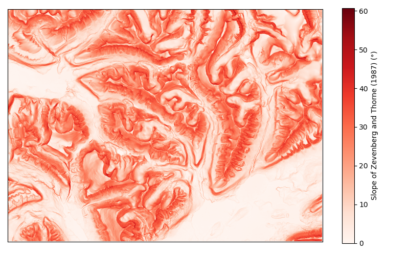
Slope with method of Zevenbergen and Thorne (1987), Equation 13.
slope_zevenberg = xdem.terrain.slope(dem, surface_fit="ZevenbergThorne")

plot_attribute(slope_zevenberg, "Reds", "Slope of Zevenberg and Thorne (1987) (°)")
Slope with method of Florinsky (2009).
slope_florinsky = xdem.terrain.slope(dem, surface_fit="Florinsky")

plot_attribute(slope_florinsky, "Reds", "Slope of Florinsky (2009) (°)")
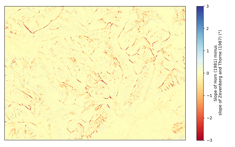
We can compute the difference between the different slope computations - for instance, here between with Horn and Zevenberg methods.
diff_slope = slope_horn - slope_zevenberg

plot_attribute(diff_slope, "RdYlBu", "Slope of Horn (1981) minus\n slope of Zevenberg and Thorne (1987) (°)", vlim=3)
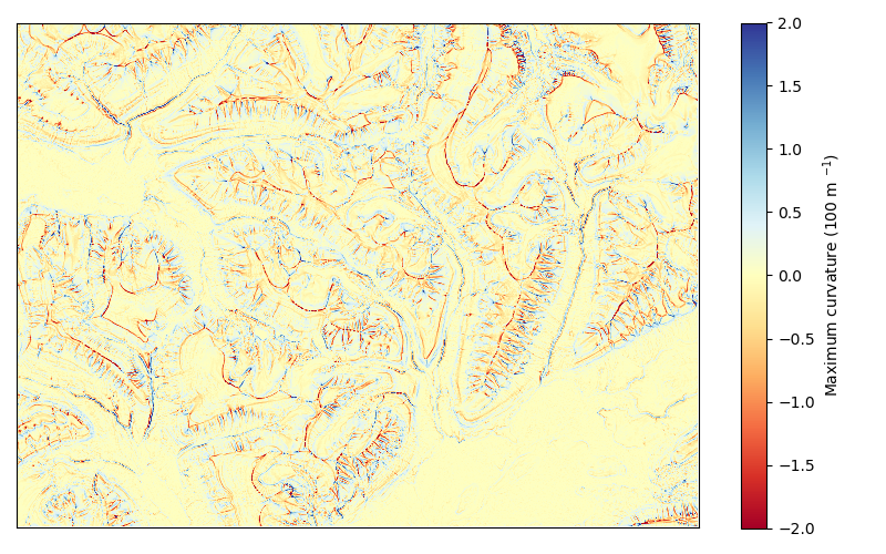
The differences are negative, implying that the method of Horn always provides flatter slopes. Additionally, they seem to occur in places of high curvatures. We verify this by plotting the maximal curvature.
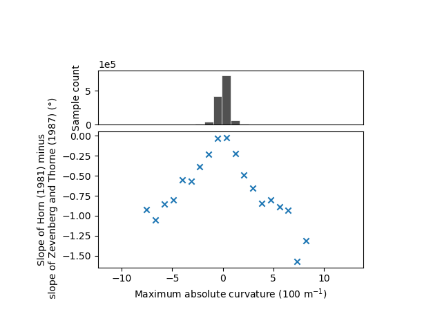
We quantify the relationship by computing the median of slope differences in bins of curvatures, and plot the result. We define custom bins for curvature, due to its skewed distribution.
df_bin = xdem.spatialstats.nd_binning(
    values=diff_slope[:],
    list_var=[maxc[:]],
    list_var_names=["maxc"],
    list_var_bins=30,
    statistics=[np.nanmedian, "count"],
)

xdem.spatialstats.plot_1d_binning(
    df_bin,
    var_name="maxc",
    statistic_name="nanmedian",
    label_var="Maximal absolute curvature (100 m$^{-1}$)",
    label_statistic="Slope of Horn (1981) minus\n " "slope of Zevenberg and Thorne (1987) (°)",
)
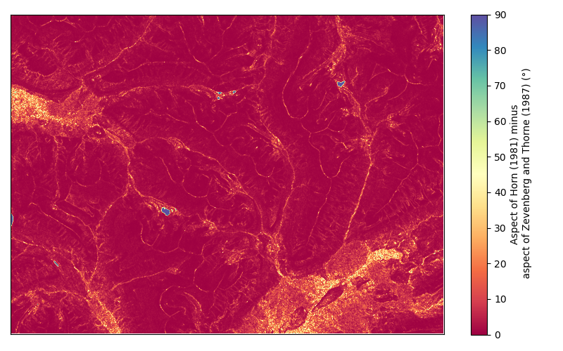
We perform the same exercise to analyze the differences in terrain aspect. We compute the difference modulo 360°, to account for the circularity of aspect.
aspect_horn = xdem.terrain.aspect(dem)
aspect_zevenberg = xdem.terrain.aspect(dem, method="ZevenbergThorne")

diff_aspect = aspect_horn - aspect_zevenberg
diff_aspect_mod = np.minimum(diff_aspect % 360, 360 - diff_aspect % 360)

plot_attribute(
    diff_aspect_mod, "Spectral", "Aspect of Horn (1981) minus\n aspect of Zevenberg and Thorne (1987) (°)", vlim=[0, 90]
)
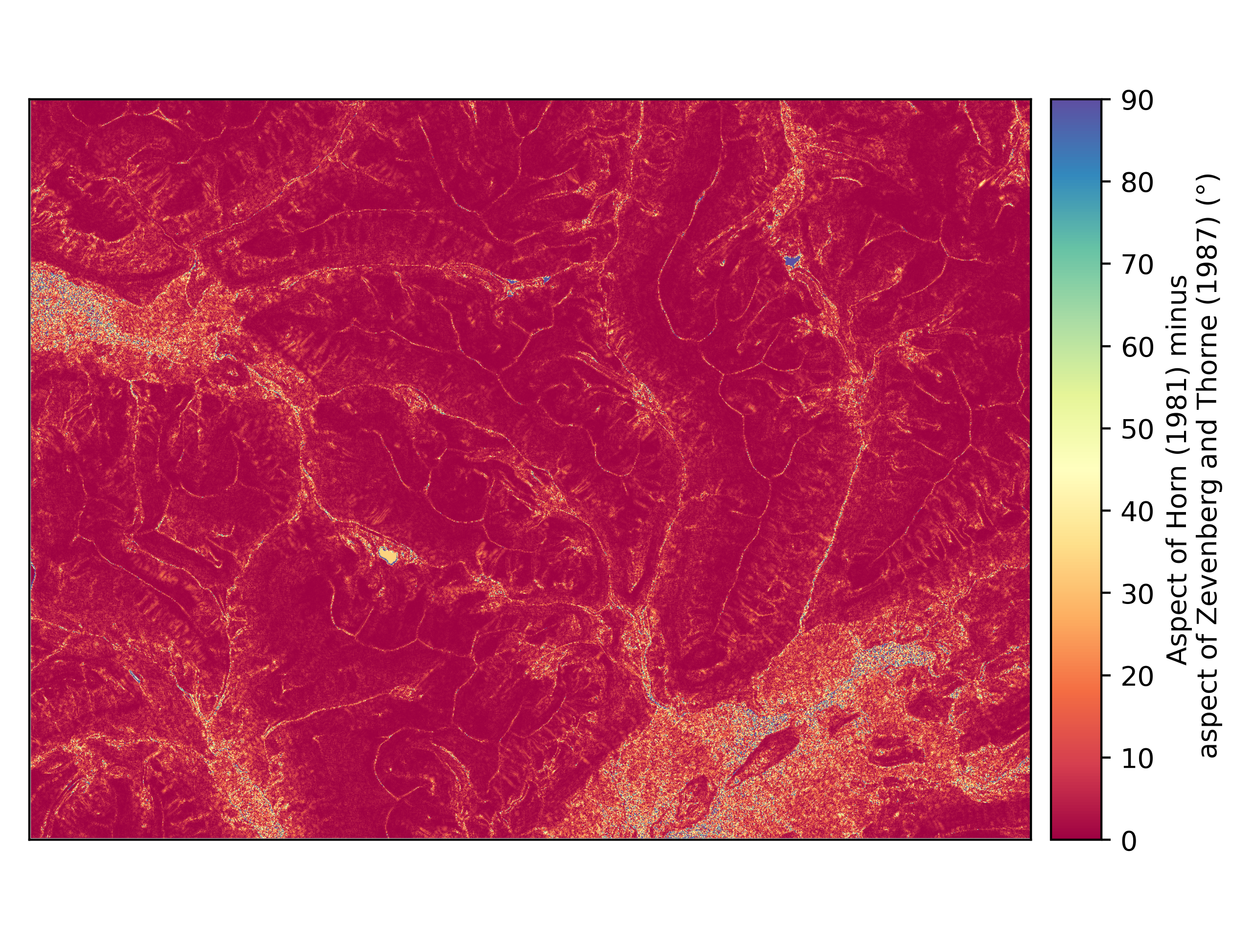
Same as for slope, differences in aspect seem to coincide with high curvature areas. We observe also observe large differences for areas with nearly flat slopes, owing to the high sensitivity of orientation estimation for flat terrain.
Note
The default aspect for a 0° slope is 180°, as in GDAL.
Total running time of the script: (0 minutes 5.889 seconds)