Note
Go to the end to download the full example code.
Spatial correlation of errors#
Digital elevation models have errors that are spatially correlated due to instrument or processing effects. Here, we rely on a non-stationary spatial statistics framework to estimate and model spatial correlations in elevation error. We use a sum of variogram forms to model this correlation, with stable terrain as an error proxy for moving terrain.
References: Rolstad et al. (2009), Hugonnet et al. (2022).
import geoutils as gu

import xdem
We load a difference of DEMs at Longyearbyen, already coregistered using Nuth and Kääb (2011) as shown in the Nuth and Kääb coregistration example. We also load the glacier outlines here corresponding to moving terrain.
dh = xdem.DEM(xdem.examples.get_path("longyearbyen_ddem"))
glacier_outlines = gu.Vector(xdem.examples.get_path("longyearbyen_glacier_outlines"))
Then, we run the pipeline for inference of elevation heteroscedasticity from stable terrain (Note: we pass a
random_state argument to ensure a fixed, reproducible random subsampling in this example). We ask for a fit with
a Gaussian model for short range (as it is passed first), and Spherical for long range (as it is passed second):
(
    df_empirical_variogram,
    df_model_params,
    spatial_corr_function,
) = xdem.spatialstats.infer_spatial_correlation_from_stable(
    dvalues=dh, list_models=["Gaussian", "Spherical"], unstable_mask=glacier_outlines, random_state=42
)
RuntimeWarning: Mean of empty slice
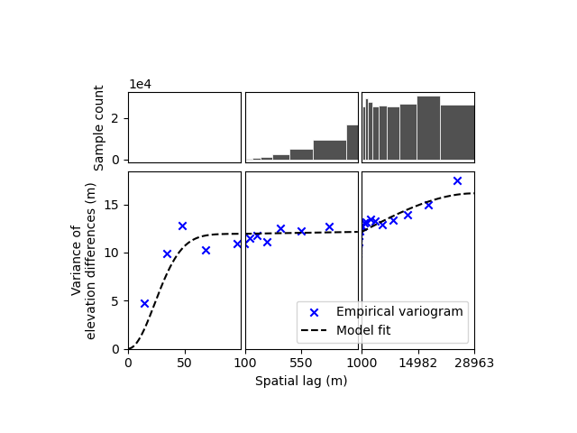
The first output corresponds to the dataframe of the empirical variogram, by default estimated using Dowd’s estimator
and a circular sampling scheme in SciKit-GStat (following Fig. S13 of Hugonnet et al. (2022)). The
lags columns is the upper bound of spatial lag bins (lower bound of first bin being 0), the exp column is the
“experimental” variance value of the variogram in that bin, the count the number of pairwise samples, and
err_exp the 1-sigma error of the “experimental” variance, if more than one variogram is estimated with the
n_variograms parameter.
df_empirical_variogram
The second output is the dataframe of optimized model parameters (range, sill, and possibly smoothness)
for a sum of gaussian and spherical models:
df_model_params
The third output is the spatial correlation function with spatial lags, derived from the variogram:
for spatial_lag in [0, 100, 1000, 10000, 30000]:
    print(
        "Errors are correlated at {:.1f}% for a {:,.0f} m spatial lag".format(
            spatial_corr_function(spatial_lag) * 100, spatial_lag
        )
    )
Errors are correlated at 100.0% for a 0 m spatial lag
Errors are correlated at 23.0% for a 100 m spatial lag
Errors are correlated at 22.0% for a 1,000 m spatial lag
Errors are correlated at 11.6% for a 10,000 m spatial lag
Errors are correlated at 0.0% for a 30,000 m spatial lag
We can plot the empirical variogram and its model on a non-linear X-axis to identify the multi-scale correlations.
xdem.spatialstats.plot_variogram(
    df=df_empirical_variogram,
    list_fit_fun=[xdem.spatialstats.get_variogram_model_func(df_model_params)],
    xlabel="Spatial lag (m)",
    ylabel="Variance of\nelevation differences (m)",
    xscale_range_split=[100, 1000],
)
This pipeline will not always work optimally with default parameters: variogram sampling is more robust with a lot of samples but takes long computing times, and the fitting might require multiple tries for forms and possibly bounds and first guesses to help the least-squares optimization. To learn how to tune more parameters and use the subfunctions, see the gallery example: Estimation and modelling of spatial variograms!
Total running time of the script: (0 minutes 6.809 seconds)