Note
Go to the end to download the full example code.
Nuth and Kääb coregistration#
The Nuth and Kääb coregistration corrects horizontal and vertical shifts, and is especially performant for precise
sub-pixel alignment in areas with varying slope.
In xDEM, this approach is implemented through the xdem.coreg.NuthKaab class.
See also the Nuth and Kääb (2011) section in feature pages.
Reference: Nuth and Kääb (2011).
import geoutils as gu
import numpy as np

import xdem
We open example files.
reference_dem = xdem.DEM(xdem.examples.get_path("longyearbyen_ref_dem"))
dem_to_be_aligned = xdem.DEM(xdem.examples.get_path("longyearbyen_tba_dem"))
glacier_outlines = gu.Vector(xdem.examples.get_path("longyearbyen_glacier_outlines"))

# We create a stable ground mask (not glacierized) to mark "inlier data".
inlier_mask = ~glacier_outlines.create_mask(reference_dem)
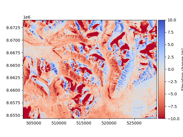
The DEM to be aligned (a 1990 photogrammetry-derived DEM) has some vertical and horizontal biases that we want to reduce. These can be visualized by plotting a change map:
diff_before = reference_dem - dem_to_be_aligned
diff_before.plot(cmap="RdYlBu", vmin=-10, vmax=10, cbar_title="Elevation change (m)")
Horizontal and vertical shifts can be estimated using NuthKaab.
The shifts are estimated then applied to the to-be-aligned elevation data:
The shifts are stored in the affine metadata output
print([nuth_kaab.meta["outputs"]["affine"][s] for s in ["shift_x", "shift_y", "shift_z"]])
[np.float64(9.174802633256634), np.float64(2.8128042041541637), -1.9848825355017254]
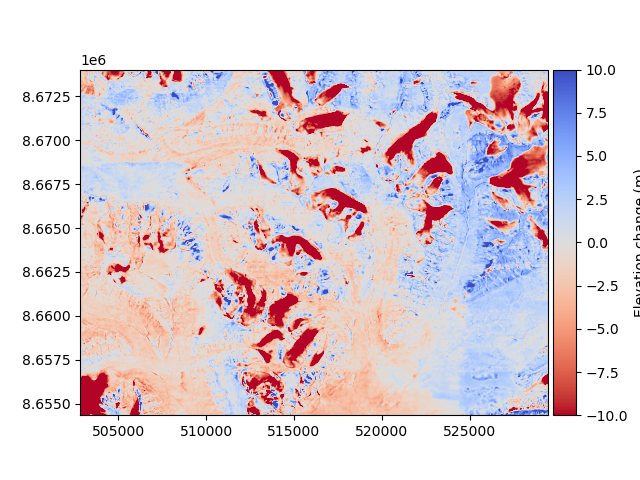
Then, the new difference can be plotted to validate that it improved.
diff_after = reference_dem - aligned_dem
diff_after.plot(cmap="RdYlBu", vmin=-10, vmax=10, cbar_title="Elevation change (m)")
We compare the median and NMAD to validate numerically that there was an improvement (see Measures of central tendency and dispersion):
inliers_before = diff_before[inlier_mask]
med_before, nmad_before = np.ma.median(inliers_before), gu.stats.nmad(inliers_before)

inliers_after = diff_after[inlier_mask]
med_after, nmad_after = np.ma.median(inliers_after), gu.stats.nmad(inliers_after)

print(f"Error before: median = {med_before:.2f} - NMAD = {nmad_before:.2f} m")
print(f"Error after: median = {med_after:.2f} - NMAD = {nmad_after:.2f} m")
Error before: median = -2.33 - NMAD = 3.42 m
Error after: median = -0.00 - NMAD = 2.51 m
In the plot above, one may notice a positive (blue) tendency toward the east. The 1990 DEM is a mosaic, and likely has a “seam” near there. Blockwise coregistration tackles this issue, using a nonlinear coregistration approach.
Total running time of the script: (0 minutes 2.746 seconds)