Terrain attributes#
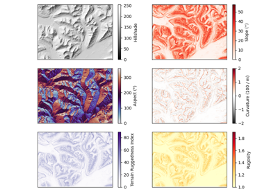
For analytic and visual purposes, deriving certain attributes of a DEM may be required. Some are useful for direct analysis, such as a slope map to differentiate features of different angles, while others, like the hillshade, are great tools for visualizing a DEM.
Slope#
xdem.terrain.slope()
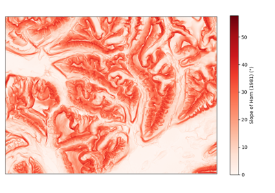
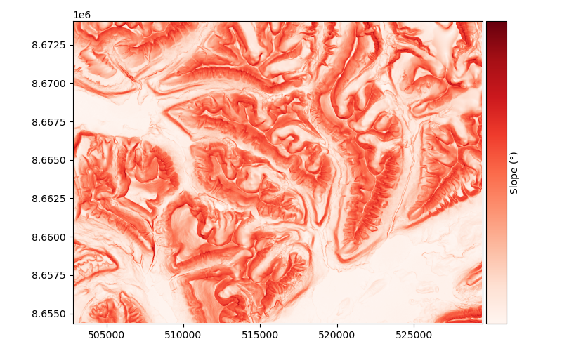
The slope of a DEM describes the tilt, or gradient, of each pixel in relation to its neighbours. It is most often described in degrees, where a flat surface is 0° and a vertical cliff is 90°. No tilt direction is stored in the slope map; a 45° tilt westward is identical to a 45° tilt eastward.
The slope can be computed either by the method of Horn (1981) (default) based on a refined gradient formulation on a 3x3 pixel window, or by the method of Zevenbergen and Thorne (1987) based on a plane fit on a 3x3 pixel window.
The differences between methods are illustrated in the Terrain attributes example.
Aspect#
xdem.terrain.aspect()
The aspect describes the orientation of strongest slope. It is often reported in degrees, where a slope tilting straight north corresponds to an aspect of 0°, and an eastern aspect is 90°, south is 180° and west is 270°. By default, a flat slope is given an arbitrary aspect of 180°.
As the aspect is directly based on the slope, it varies between the method of Horn (1981) (default) and that of Zevenbergen and Thorne (1987).
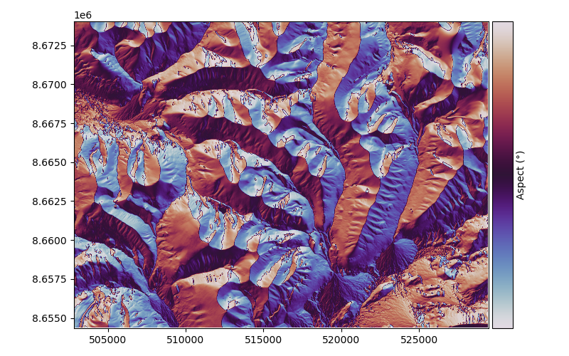
Examples using xdem.terrain.aspect#
Hillshade#
xdem.terrain.hillshade()
The hillshade is a slope map, shaded by the aspect of the slope. The slope map is a good tool to visualize terrain, but it does not distinguish between a mountain and a valley. It may therefore be slightly difficult to interpret in mountainous terrain. Hillshades are therefore often preferable for visualizing DEMs. With a westerly azimuth (a simulated sun coming from the west), all eastern slopes are slightly darker. This mode of shading the slopes often generates a map that is much more easily interpreted than the slope map.
As the hillshade is directly based on the slope and aspect, it varies between the method of Horn (1981) (default) and that of Zevenbergen and Thorne (1987).
Note, however, that the hillshade is not a shadow map; no occlusion is taken into account so it does not represent “true” shading. It therefore has little analytic purpose, but it still constitutes a great visualization tool.
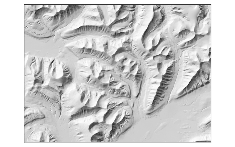
Examples using xdem.terrain.hillshade#
Curvature#
xdem.terrain.curvature()
The curvature map is the second derivative of elevation, which highlights the convexity or concavity of the terrain. If a surface is convex (like a mountain peak), it will have positive curvature. If a surface is concave (like a through or a valley bottom), it will have negative curvature. The curvature values in units of m-1 are quite small, so they are by convention multiplied by 100.
The curvature is based on the method of Zevenbergen and Thorne (1987).
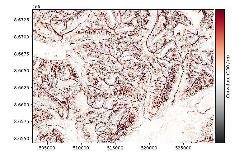
Examples using xdem.terrain.curvature#
Planform curvature#
xdem.terrain.planform_curvature()
The planform curvature is the curvature perpendicular to the direction of slope, reported in 100 m-1.
It is based on the method of Zevenbergen and Thorne (1987).
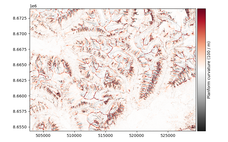
Examples using xdem.terrain.planform_curvature#
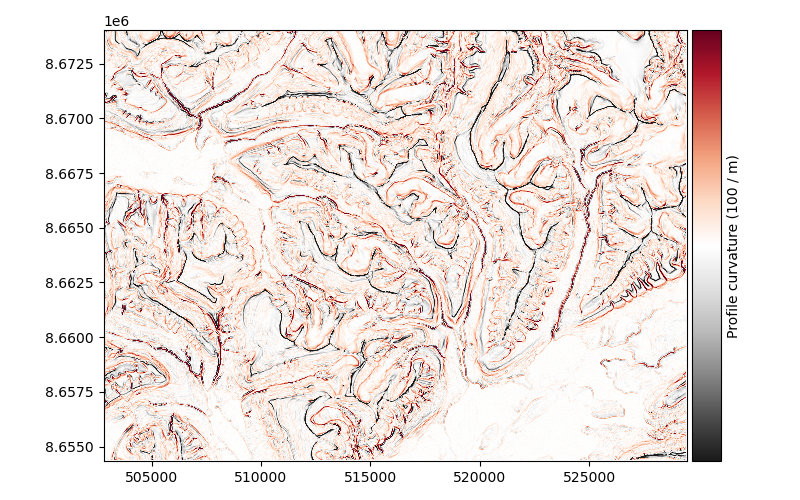
Profile curvature#
xdem.terrain.profile_curvature()
The profile curvature is the curvature parallel to the direction of slope, reported in 100 m-1..
It is based on the method of Zevenbergen and Thorne (1987).
Examples using xdem.terrain.profile_curvature#
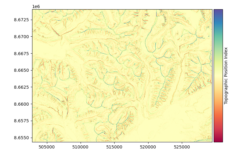
Topographic Position Index#
xdem.terrain.topographic_position_index()
The Topographic Position Index (TPI) is a metric of slope position, based on the method of Weiss (2001) that corresponds to the difference of the elevation of a central pixel with the average of that of neighbouring pixels. Its unit is that of the DEM (typically meters) and it can be computed for any window size (default 3x3 pixels).
Examples using xdem.terrain.topographic_position_index#
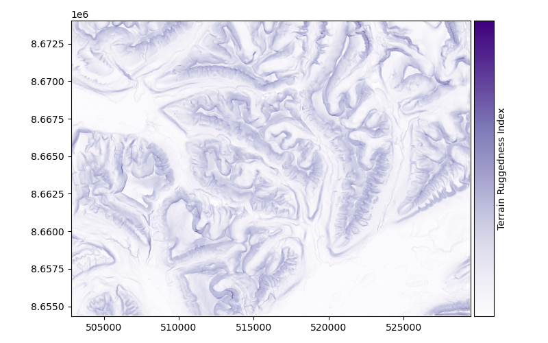
Terrain Ruggedness Index#
xdem.terrain.terrain_ruggedness_index()
The Terrain Ruggedness Index (TRI) is a metric of terrain ruggedness, based on cumulated differences in elevation between a central pixel and its surroundings. Its unit is that of the DEM (typically meters) and it can be computed for any window size (default 3x3 pixels).
For topography (default), the method of Riley et al. (1999) is generally used, where the TRI is computed by the squareroot of squared differences with neighbouring pixels.
For bathymetry, the method of Wilson et al. (2007) is generally used, where the TRI is defined by the mean absolute difference with neighbouring pixels
Examples using xdem.terrain.terrain_ruggedness_index#
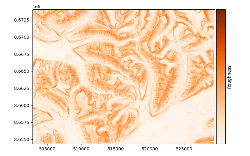
Roughness#
xdem.terrain.roughness()
The roughness is a metric of terrain ruggedness, based on the maximum difference in elevation in the surroundings. The roughness is based on the method of Dartnell (2000). Its unit is that of the DEM (typically meters) and it can be computed for any window size (default 3x3 pixels).
Examples using xdem.terrain.roughness#
Rugosity#
xdem.terrain.rugosity()
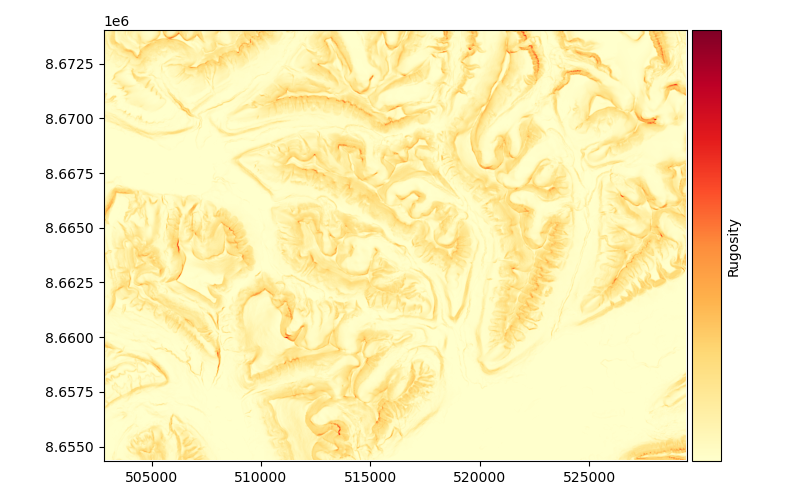
The rugosity is a metric of terrain ruggedness, based on the ratio between planimetric and real surface area. The rugosity is based on the method of Jenness (2004). It is unitless, and is only supported for a 3x3 window size.
Examples using xdem.terrain.rugosity#
Fractal roughness#
xdem.terrain.fractal_roughness()
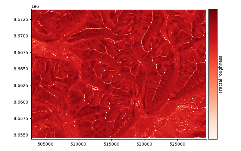
The fractal roughness is a metric of terrain ruggedness based on the local fractal dimension estimated by the volume box-counting method of Taud and Parrot (2005). The fractal roughness is computed by estimating the fractal dimension in 3D space, for a local window centered on the DEM pixels. Its unit is that of a dimension, and is always between 1 (dimension of a line in 3D space) and 3 (dimension of a cube in 3D space). It can only be computed on window sizes larger than 5x5 pixels, and defaults to 13x13.
Examples using xdem.terrain.fractal_roughness#
Generating multiple attributes at once#
Often, one may seek more terrain attributes than one, e.g. both the slope and the aspect.
Since both are dependent on the gradient of the DEM, calculating them separately is computationally repetitive.
Multiple terrain attributes can be calculated from the same gradient using the xdem.terrain.get_terrain_attribute() function.
