Note
Go to the end to download the full example code.
Elevation error map#
Digital elevation models have a precision that can vary with terrain and instrument-related variables. Here, we rely on a non-stationary spatial statistics framework to estimate and model this variability in elevation error, using terrain slope and maximum curvature as explanatory variables, with stable terrain as an error proxy for moving terrain.
Reference: Hugonnet et al. (2022).
import geoutils as gu

import xdem
We load a difference of DEMs at Longyearbyen, already coregistered using Nuth and Kääb (2011) as shown in the Nuth and Kääb coregistration example. We also load the reference DEM to derive terrain attributes and the glacier outlines here corresponding to moving terrain.
We derive the terrain slope and max curvature from the reference DEM.
slope, max_curvature = xdem.terrain.get_terrain_attribute(ref_dem, attribute=["slope", "max_curvature"])
Then, we run the pipeline for inference of elevation heteroscedasticity from stable terrain:
errors, df_binning, error_function = xdem.spatialstats.infer_heteroscedasticity_from_stable(
    dvalues=dh, list_var=[slope, max_curvature], list_var_names=["slope", "maxc"], unstable_mask=glacier_outlines
)
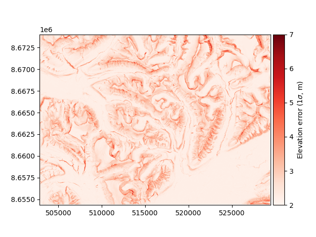
The first output corresponds to the error map for the DEM (\(\pm\) 1\(\sigma\) level):
errors.plot(vmin=2, vmax=7, cmap="Reds", cbar_title=r"Elevation error (1$\sigma$, m)")
The second output is the dataframe of 2D binning with slope and max curvature:
df_binning
The third output is the 2D binning interpolant, i.e. an error function with the slope and max curvature (Note: below we divide the max curvature by 100 to convert it in m-1 ):
Error for a slope of 0 degrees and 0.00 m-1 max. curvature: 2.2 m
Error for a slope of 40 degrees and 0.00 m-1 max. curvature: 4.1 m
Error for a slope of 0 degrees and 0.05 m-1 max. curvature: 2.4 m
Error for a slope of 40 degrees and 0.05 m-1 max. curvature: 5.1 m
This pipeline will not always work optimally with default parameters: spread estimates can be affected by skewed distributions, the binning by extreme range of values, some DEMs do not have any error variability with terrain (e.g., terrestrial photogrammetry). To learn how to tune more parameters and use the subfunctions, see the gallery example: Estimation and modelling of heteroscedasticity!
Total running time of the script: (0 minutes 2.246 seconds)