Working with a collection of DEMs

Oftentimes, more than two timestamps (DEMs) are analyzed simultaneously. One single dDEM only captures one interval, so multiple dDEMs have to be created. In addition, if multiple masking polygons exist (e.g. glacier outlines from multiple years), these should be accounted for properly. The xdem.DEMCollection is a tool to properly work with multiple timestamps at the same time, and makes calculations of elevation/volume change over multiple years easy.

from datetime import datetime

import geoutils as gu
import matplotlib.pyplot as plt

import xdem

Example data.

We can load the DEMs as usual, but with the addition that the datetime argument should be filled. Since multiple DEMs are in question, the “time dimension” is what keeps them apart.

dem_2009 = xdem.DEM(xdem.examples.get_path("longyearbyen_ref_dem"), datetime=datetime(2009, 8, 1))
dem_1990 = xdem.DEM(xdem.examples.get_path("longyearbyen_tba_dem"), datetime=datetime(1990, 8, 1))

For glacier research (any many other fields), only a subset of the DEMs are usually interesting. These parts can be delineated with masks or polygons. Here, we have glacier outlines from 1990 and 2009.

outlines = {
    datetime(1990, 8, 1): gu.Vector(xdem.examples.get_path("longyearbyen_glacier_outlines")),
    datetime(2009, 8, 1): gu.Vector(xdem.examples.get_path("longyearbyen_glacier_outlines_2010")),
}

To experiment with a longer time-series, we can also fake a 2060 DEM, by simply exaggerating the 1990-2009 change.

# Fake a 2060 DEM by assuming twice the change from 1990-2009 between 2009 and 2060
dem_2060 = dem_2009 + (dem_2009 - dem_1990).data * 3
dem_2060.datetime = datetime(2060, 8, 1)

Now, all data are ready to be collected in an xdem.DEMCollection object. What we have are: 1. Three DEMs from 1990, 2009, and 2060 (the last is artificial) 2. Two glacier outline timestamps from 1990 and 2009

demcollection = xdem.DEMCollection(dems=[dem_1990, dem_2009, dem_2060], outlines=outlines, reference_dem=1)

We can generate xdem.dDEM objects using xdem.DEMCollection.subtract_dems(). In this case, it will generate three dDEMs:

• 1990-2009

• 2009-2009 (to maintain the dems and ddems list length and order)

• 2060-2009 (note the inverted order; negative change will be positive)

_ = demcollection.subtract_dems()

These are saved internally, but are also returned as a list.

An elevation or volume change series can automatically be generated from the DEMCollection. In this case, we should specify which glacier we want the change for, as a regional value may not always be required. We can look at the glacier called “Scott Turnerbreen”, specified in the “NAME” column of the outline data. See here for the outline filtering syntax.

demcollection.get_cumulative_series(kind="dh", outlines_filter="NAME == 'Scott Turnerbreen'")

1990-08-01     0.000000
2009-08-01   -13.379259
2060-08-01   -51.885126
dtype: float64

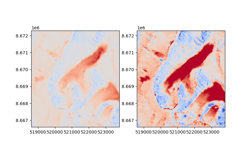
And there we have a cumulative dH series of the glacier Scott Turnerbreen on Svalbard! The dDEMs can be visualized to give further context.

extent = [
    demcollection.dems[0].bounds.left,
    demcollection.dems[0].bounds.right,
    demcollection.dems[0].bounds.bottom,
    demcollection.dems[0].bounds.top,
]

scott_extent = [518600, 523800, 8666600, 8672300]

plt.figure(figsize=(8, 5))

for i in range(2):
    plt.subplot(1, 2, i + 1)

    if i == 0:
        title = "1990 - 2009"
        ddem_2060 = demcollection.ddems[0].data.squeeze()
    else:
        title = "2009 - 2060"
        # The 2009 - 2060 DEM is inverted since the reference year is 2009
        ddem_2060 = -demcollection.ddems[2].data.squeeze()

    plt.imshow(ddem_2060, cmap="coolwarm_r", vmin=-50, vmax=50, extent=extent)
    plt.xlim(scott_extent[:2])
    plt.ylim(scott_extent[2:])

plt.show()