Iterative closest point coregistration

Iterative closest point (ICP) is a registration method accounting for both rotations and translations.

It is used primarily to correct rotations, as it generally performs worse than Nuth and Kääb (2011) for sub-pixel shifts. Fortunately, xDEM provides the best of two worlds by allowing a combination of the two methods in a pipeline, demonstrated below!

References: Besl and McKay (1992).

import matplotlib.pyplot as plt
import numpy as np

import xdem

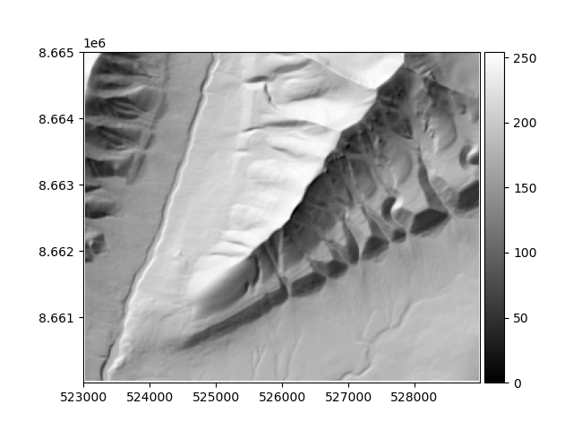
We load a DEM and crop it to a single mountain on Svalbard, called Battfjellet. Its aspects vary in every direction, and is therefore a good candidate for coregistration exercises.

dem = xdem.DEM(xdem.examples.get_path("longyearbyen_ref_dem"))

subset_extent = [523000, 8660000, 529000, 8665000]
dem = dem.crop(subset_extent)

Let’s plot a hillshade of the mountain for context.

xdem.terrain.hillshade(dem).plot(cmap="gray")

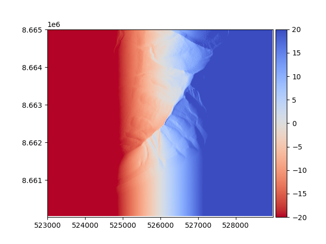
To try the effects of rotation, we can artificially rotate the DEM using a transformation matrix. Here, a rotation of just one degree is attempted. But keep in mind: the window is 6 km wide; 1 degree of rotation at the center equals to a 52 m vertical difference at the edges!

rotation = np.deg2rad(1)
rotation_matrix = np.array(
    [
        [np.cos(rotation), 0, np.sin(rotation), 0],
        [0, 1, 0, 0],
        [-np.sin(rotation), 0, np.cos(rotation), 0],
        [0, 0, 0, 1],
    ]
)
centroid = [dem.bounds.left + dem.width / 2, dem.bounds.bottom + dem.height / 2, np.nanmean(dem)]
# This will apply the matrix along the center of the DEM
rotated_dem = xdem.coreg.apply_matrix(dem, matrix=rotation_matrix, centroid=centroid)

We can plot the difference between the original and rotated DEM. It is now artificially tilting from east down to the west.

diff_before = dem - rotated_dem
diff_before.plot(cmap="RdYlBu", vmin=-20, vmax=20, cbar_title="Elevation differences (m)")
plt.show()

As previously mentioned, NuthKaab works well on sub-pixel scale but does not handle rotation. ICP works with rotation but lacks the sub-pixel accuracy. Luckily, these can be combined! Any xdem.coreg.Coreg subclass can be added with another, making a xdem.coreg.CoregPipeline. With a pipeline, each step is run sequentially, potentially leading to a better result. Let’s try all three approaches: ICP, NuthKaab and ICP + NuthKaab.

approaches = [
    (xdem.coreg.ICP(), "ICP"),
    (xdem.coreg.NuthKaab(), "NuthKaab"),
    (xdem.coreg.ICP() + xdem.coreg.NuthKaab(), "ICP + NuthKaab"),
]


plt.figure(figsize=(6, 12))

for i, (approach, name) in enumerate(approaches):
    corrected_dem = approach.fit_and_apply(
        reference_elev=dem,
        to_be_aligned_elev=rotated_dem,
    )

    diff = dem - corrected_dem

    ax = plt.subplot(3, 1, i + 1)
    plt.title(name)
    diff.plot(cmap="RdYlBu", vmin=-20, vmax=20, ax=ax, cbar_title="Elevation differences (m)")

plt.tight_layout()
plt.show()

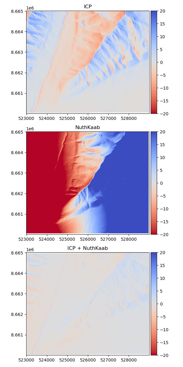
The results show what we expected:

• ICP alone handled the rotational offset, but left a horizontal offset as it is not sub-pixel accurate (in this case, the resolution is 20x20m).

• Nuth and Kääb barely helped at all, since the offset is purely rotational.

• ICP + Nuth and Kääb first handled the rotation, then fit the reference with sub-pixel accuracy.

The last result is an almost identical raster that was offset but then corrected back to its original position!