Note
Go to the end to download the full example code.
Estimation and modelling of heteroscedasticity#
Digital elevation models have a precision that can vary with terrain and instrument-related variables. This variability in variance is called heteroscedasticy, and rarely accounted for in DEM studies (see Grasping accuracy and precision). Quantifying elevation heteroscedasticity is essential to use stable terrain as an error proxy for moving terrain, and standardize data towards a stationary variance, necessary to apply spatial statistics (see Uncertainty analysis).
Here, we show an advanced example in which we look for terrain-dependent explanatory variables to explain the
heteroscedasticity for a DEM difference at Longyearbyen. We detail the steps used by
infer_heteroscedasticity_from_stable() exemplified in Elevation error map.
We use data binning and robust statistics in N-dimension with
nd_binning(), apply a N-dimensional interpolation with
interp_nd_binning(), and scale our interpolant function with a two-step standardization
two_step_standardization() to produce the final elevation error function.
Reference: Hugonnet et al. (2022).
import geoutils as gu

import numpy as np

import xdem
We load example files and create a glacier mask.
ref_dem = xdem.DEM(xdem.examples.get_path("longyearbyen_ref_dem"))
dh = xdem.DEM(xdem.examples.get_path("longyearbyen_ddem"))
glacier_outlines = gu.Vector(xdem.examples.get_path("longyearbyen_glacier_outlines"))
mask_glacier = glacier_outlines.create_mask(dh)
We derive terrain attributes from the reference DEM (see Terrain attributes), which we will use to explore the variability in elevation error.
We convert to arrays and keep only stable terrain for the analysis of variability
dh_arr = dh[~mask_glacier].filled(np.nan)
slope_arr = slope[~mask_glacier].filled(np.nan)
aspect_arr = aspect[~mask_glacier].filled(np.nan)
planc_arr = planc[~mask_glacier].filled(np.nan)
profc_arr = profc[~mask_glacier].filled(np.nan)
We use xdem.spatialstats.nd_binning() to perform N-dimensional binning on all those terrain variables, with uniform
bin length divided by 30. We use the NMAD as a robust measure of statistical dispersion
(see Measures of central tendency and dispersion).
df = xdem.spatialstats.nd_binning(
    values=dh_arr,
    list_var=[slope_arr, aspect_arr, planc_arr, profc_arr],
    list_var_names=["slope", "aspect", "planc", "profc"],
    statistics=["count", gu.stats.nmad],
    list_var_bins=30,
)
We obtain a dataframe with the 1D binning results for each variable, the 2D binning results for all combinations of variables and the N-D (here 4D) binning with all variables. Overview of the dataframe structure for the 1D binning:
df[df.nd == 1]
And for the 4D binning:
df[df.nd == 4]
We can now visualize the results of the 1D binning of the computed NMAD of elevation differences with each variable
using xdem.spatialstats.plot_1d_binning().
We can start with the slope that has been long known to be related to the elevation measurement error (e.g.,
Toutin (2002)).
xdem.spatialstats.plot_1d_binning(
    df, var_name="slope", statistic_name="nmad", label_var="Slope (degrees)", label_statistic="NMAD of dh (m)"
)
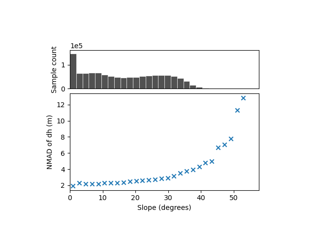
We identify a clear variability, with the dispersion estimated from the NMAD increasing from ~2 meters for nearly flat slopes to above 12 meters for slopes steeper than 50°.
What about the aspect?
xdem.spatialstats.plot_1d_binning(df, "aspect", "nmad", "Aspect (degrees)", "NMAD of dh (m)")
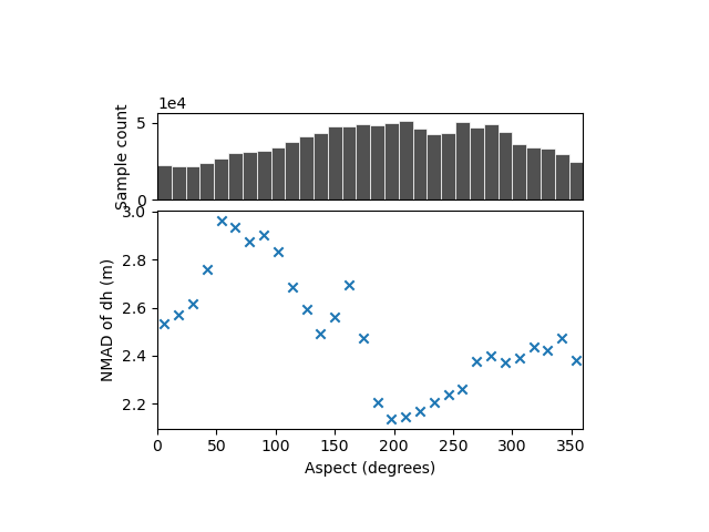
There is no variability with the aspect that shows a dispersion averaging 2-3 meters, i.e. that of the complete sample.
What about the plan curvature?
xdem.spatialstats.plot_1d_binning(df, "planc", "nmad", "Planform curvature (100 m$^{-1}$)", "NMAD of dh (m)")
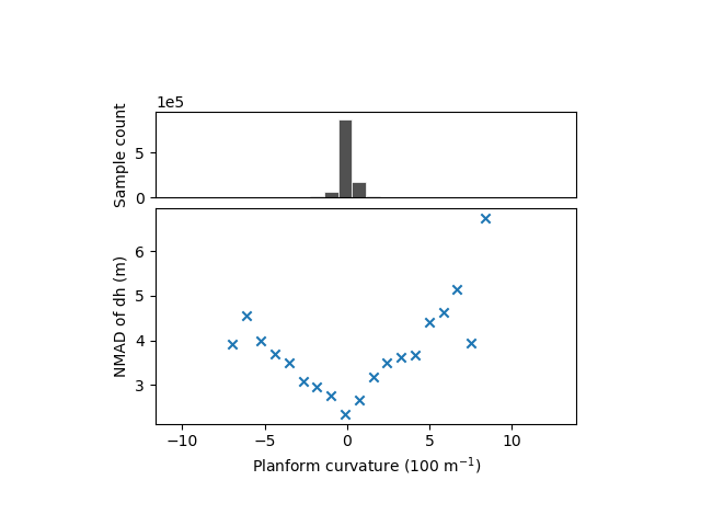
The relation with the plan curvature remains ambiguous.
We should better define our bins to avoid sampling bins with too many or too few samples. For this, we can partition
the data in quantiles in xdem.spatialstats.nd_binning(). We define 1000 quantile bins of size
0.001 (equivalent to 0.1% percentile bins) for the profile curvature:
Note
We need a higher number of bins to work with quantiles and still resolve the edges of the distribution.
df = xdem.spatialstats.nd_binning(
    values=dh_arr,
    list_var=[profc_arr],
    list_var_names=["profc"],
    statistics=["count", np.nanmedian, gu.stats.nmad],
    list_var_bins=[np.nanquantile(profc_arr, np.linspace(0, 1, 1000))],
)
xdem.spatialstats.plot_1d_binning(df, "profc", "nmad", "Profile curvature (100 m$^{-1}$)", "NMAD of dh (m)")
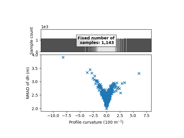
We clearly identify a variability with the profile curvature, from 2 meters for low curvatures to above 4 meters for higher positive or negative curvature.
What about the role of the plan curvature?
df = xdem.spatialstats.nd_binning(
    values=dh_arr,
    list_var=[planc_arr],
    list_var_names=["planc"],
    statistics=["count", np.nanmedian, gu.stats.nmad],
    list_var_bins=[np.nanquantile(planc_arr, np.linspace(0, 1, 1000))],
)
xdem.spatialstats.plot_1d_binning(df, "planc", "nmad", "Planform curvature (100 m$^{-1}$)", "NMAD of dh (m)")
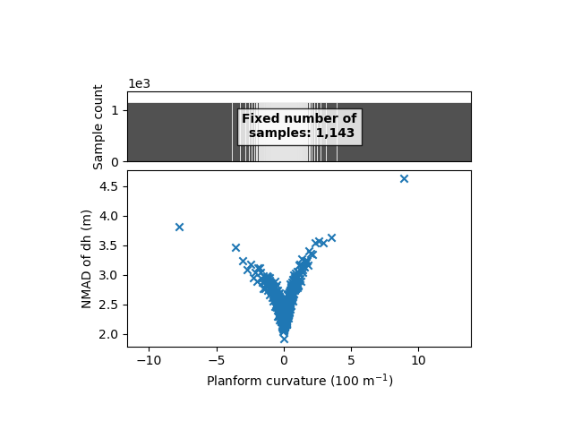
The plan curvature shows a similar relation. Those are symmetrical with 0, and almost equal for both types of curvature. To simplify the analysis, we here combine those curvatures into the maximum absolute curvature:
maxc_arr = np.maximum(np.abs(planc_arr), np.abs(profc_arr))
df = xdem.spatialstats.nd_binning(
    values=dh_arr,
    list_var=[maxc_arr],
    list_var_names=["maxc"],
    statistics=["count", np.nanmedian, gu.stats.nmad],
    list_var_bins=[np.nanquantile(maxc_arr, np.linspace(0, 1, 1000))],
)
xdem.spatialstats.plot_1d_binning(df, "maxc", "nmad", "Maximum absolute curvature (100 m$^{-1}$)", "NMAD of dh (m)")
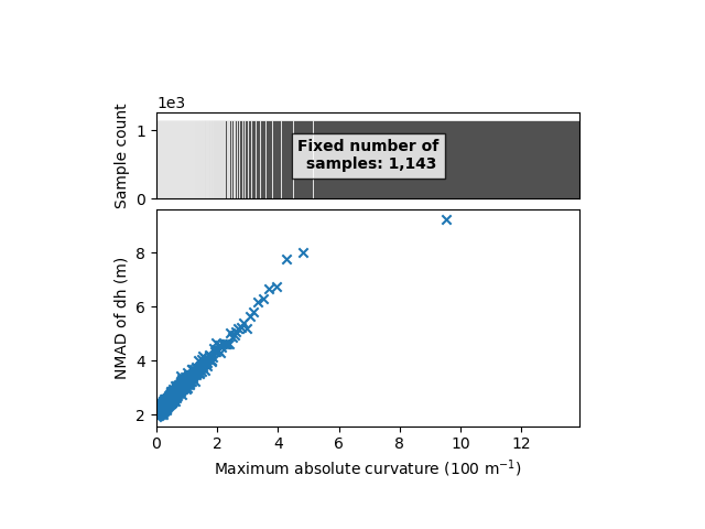
Here’s our simplified relation! We now have both slope and maximum absolute curvature with clear variability of the elevation error.
But, one might wonder: high curvatures might occur more often around steep slopes than flat slope, so what if those two dependencies are actually one and the same?
We need to explore the variability with both slope and curvature at the same time:
df = xdem.spatialstats.nd_binning(
    values=dh_arr,
    list_var=[slope_arr, maxc_arr],
    list_var_names=["slope", "maxc"],
    statistics=["count", np.nanmedian, gu.stats.nmad],
    list_var_bins=30,
)

xdem.spatialstats.plot_2d_binning(
    df,
    var_name_1="slope",
    var_name_2="maxc",
    statistic_name="nmad",
    label_var_name_1="Slope (degrees)",
    label_var_name_2="Maximum absolute curvature (100 m$^{-1}$)",
    label_statistic="NMAD of dh (m)",
)
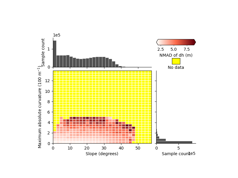
We can see that part of the variability seems to be independent, but with the uniform bins it is hard to tell much more.
If we use custom quantiles for both binning variables, and adjust the plot scale:
custom_bin_slope = np.unique(
    np.concatenate(
        [
            np.nanquantile(slope_arr, np.linspace(0, 0.95, 20)),
            np.nanquantile(slope_arr, np.linspace(0.96, 0.99, 5)),
            np.nanquantile(slope_arr, np.linspace(0.991, 1, 10)),
        ]
    )
)

custom_bin_curvature = np.unique(
    np.concatenate(
        [
            np.nanquantile(maxc_arr, np.linspace(0, 0.95, 20)),
            np.nanquantile(maxc_arr, np.linspace(0.96, 0.99, 5)),
            np.nanquantile(maxc_arr, np.linspace(0.991, 1, 10)),
        ]
    )
)

df = xdem.spatialstats.nd_binning(
    values=dh_arr,
    list_var=[slope_arr, maxc_arr],
    list_var_names=["slope", "maxc"],
    statistics=["count", np.nanmedian, gu.stats.nmad],
    list_var_bins=[custom_bin_slope, custom_bin_curvature],
)
xdem.spatialstats.plot_2d_binning(
    df,
    "slope",
    "maxc",
    "nmad",
    "Slope (degrees)",
    "Maximum absolute curvature (100 m$^{-1}$)",
    "NMAD of dh (m)",
    scale_var_2="log",
    vmin=2,
    vmax=10,
)
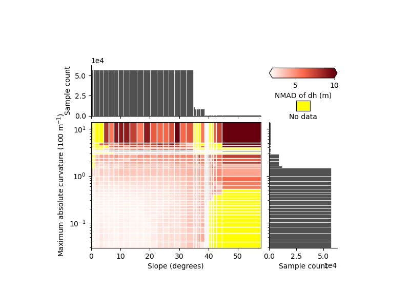
We identify clearly that the two variables have an independent effect on the precision, with
high curvatures and flat slopes that have larger errors than low curvatures and flat slopes
steep slopes and low curvatures that have larger errors than low curvatures and flat slopes as well
We also identify that, steep slopes (> 40°) only correspond to high curvature, while the opposite is not true, hence the importance of mapping the variability in two dimensions.
Now we need to account for the heteroscedasticity identified. For this, the simplest approach is a numerical
approximation i.e. a piecewise linear interpolation/extrapolation based on the binning results available through
the function xdem.spatialstats.interp_nd_binning(). To ensure that only robust statistic values are used
in the interpolation, we set a min_count value at 30 samples.
unscaled_dh_err_fun = xdem.spatialstats.interp_nd_binning(
    df, list_var_names=["slope", "maxc"], statistic="nmad", min_count=30
)
The output is an interpolant function of slope and curvature that predicts the elevation error at any point. However, this predicted error might have a spread slightly off from that of the data:
We compare the spread of the elevation difference on stable terrain and the average predicted error:
dh_err_stable = unscaled_dh_err_fun((slope_arr, maxc_arr))

print(
    "The spread of elevation difference is {:.2f} "
    "compared to a mean predicted elevation error of {:.2f}.".format(gu.stats.nmad(dh_arr), np.nanmean(dh_err_stable))
)
The spread of elevation difference is 2.51 compared to a mean predicted elevation error of 2.55.
Thus, we rescale the function to exactly match the spread on stable terrain using the
xdem.spatialstats.two_step_standardization() function, and get our final error function.
zscores, dh_err_fun = xdem.spatialstats.two_step_standardization(
    dh_arr, list_var=[slope_arr, maxc_arr], unscaled_error_fun=unscaled_dh_err_fun
)

for s, c in [(0.0, 0.1), (50.0, 0.1), (0.0, 20.0), (50.0, 20.0)]:
    print(
        "Elevation measurement error for slope of {:.0f} degrees, "
        "curvature of {:.2f} m-1: {:.1f}".format(s, c / 100, dh_err_fun((s, c))) + " meters."
    )
Elevation measurement error for slope of 0 degrees, curvature of 0.00 m-1: 2.2 meters.
Elevation measurement error for slope of 50 degrees, curvature of 0.00 m-1: 5.7 meters.
Elevation measurement error for slope of 0 degrees, curvature of 0.20 m-1: 2.3 meters.
Elevation measurement error for slope of 50 degrees, curvature of 0.20 m-1: 6.8 meters.
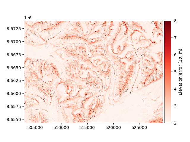
This function can be used to estimate the spatial distribution of the elevation error on the extent of our DEMs:
maxc = np.maximum(np.abs(profc), np.abs(planc))
errors = dh.copy(new_array=dh_err_fun((slope.data, maxc.data)))

errors.plot(cmap="Reds", vmin=2, vmax=8, cbar_title=r"Elevation error ($1\sigma$, m)")
Total running time of the script: (0 minutes 32.496 seconds)