Coregistration

xDEM implements a wide range of coregistration algorithms and pipelines for 3-dimensional alignment from the peer-reviewed literature often tailored specifically to elevation data, aiming at correcting systematic elevation errors.

Two categories of alignment are generally differentiated: 3D affine transformations described below, and other alignments that possibly rely on external variables, described in Bias correction.

Affine transformations can include vertical and horizontal translations, rotations and reflections, and scalings.

More reading

Coregistration heavily relies on the use of static surfaces, which you can read more about on the Static surfaces as error proxy guide page.

Quick use

Coregistration pipelines are defined by combining Coreg objects:

import xdem

# Create a coregistration pipeline
my_coreg_pipeline = xdem.coreg.ICP() + xdem.coreg.NuthKaab()

# Or use a single method
my_coreg_pipeline = xdem.coreg.NuthKaab()

Then, coregistering a pair of elevation data can be done by calling coregister_3d() from the xdem.DEM or xdem.EPC that should be aligned.

Show the code for opening example files

Hide the code for opening example files

import geoutils as gu
import numpy as np
import matplotlib.pyplot as plt

# Open a reference and to-be-aligned DEM
ref_dem = xdem.DEM(xdem.examples.get_path("longyearbyen_ref_dem"))
tba_dem = xdem.DEM(xdem.examples.get_path("longyearbyen_tba_dem"))

# Coregister by calling the DEM or EPC method
aligned_dem = tba_dem.coregister_3d(ref_dem, my_coreg_pipeline)

Alternatively, the coregistration can be applied by calling fit_and_apply(), or sequentially calling the fit() and apply() steps, which allows a broader variety of arguments at each step, and reusing the same transformation on several objects (e.g., horizontal shift of both a stereo DEM and its ortho-image).

# (Equivalent) Or use fit and apply
aligned_dem = my_coreg_pipeline.fit_and_apply(ref_dem, tba_dem)

Information about the coregistration inputs and outputs is summarized in info().

Tip

Often, an inlier_mask has to be passed to fit() to isolate static surfaces to utilize during coregistration (for instance removing vegetation, snow, glaciers). This mask can be easily derived using create_mask().

Summary of supported methods

Affine method	Description	Reference
Nuth and Kääb (2011)	Translations	Nuth and Kääb (2011)
Minimization of dh	Translations	N/A
Least Z-difference	Translations and rotations	Rosenholm and Torlegård (1988)
Iterative closest point	Translations and rotations	Besl and McKay (1992), Chen and Medioni (1992)
Coherent point drift	Translations and rotations	Myronenko and Song (2010)
Vertical shift	Vertical translation	N/A

Using a coregistration

The Coreg object

Each coregistration method implemented in xDEM inherits their interface from the Coreg class¹, and has the following methods:

• fit_and_apply() for estimating the transformation and applying it in one step,

• info() for plotting the metadata, including inputs and outputs of the coregistration.

For more details on the input and output metadata stored by coregistration methods, see the Coregistration metadata section.

The two above methods cover most uses. More specific methods are also available:

• fit() for estimating the transformation without applying it,

• apply() for applying an estimated transformation,

• to_matrix() to convert the transform to a 4x4 transformation matrix, if possible,

• from_matrix() to create a coregistration from a 4x4 transformation matrix.

¹In a style inspired by scikit-learn’s pipelines.

Inheritance diagram of implemented coregistrations:

See Bias correction for more information on non-rigid transformations.

Coregistration methods

Important

Below we create misaligned elevation data to examplify the different methods in relation to their type of affine transformation.

See coregistration on real data in the Basic and Advanced gallery examples!

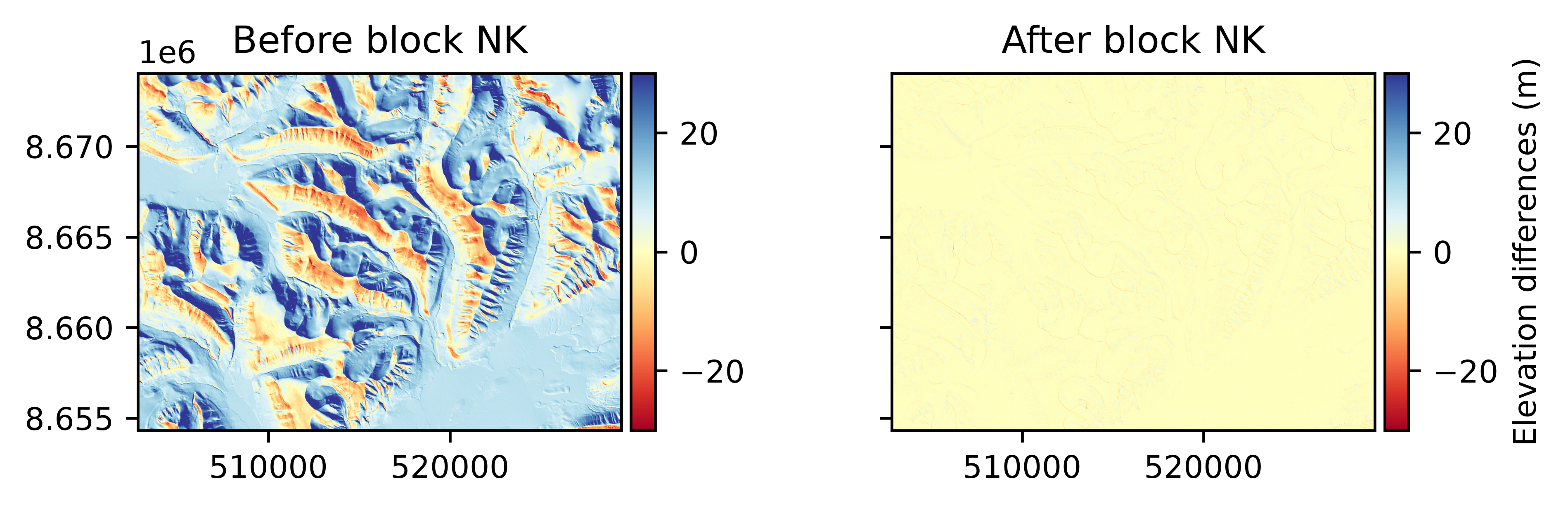
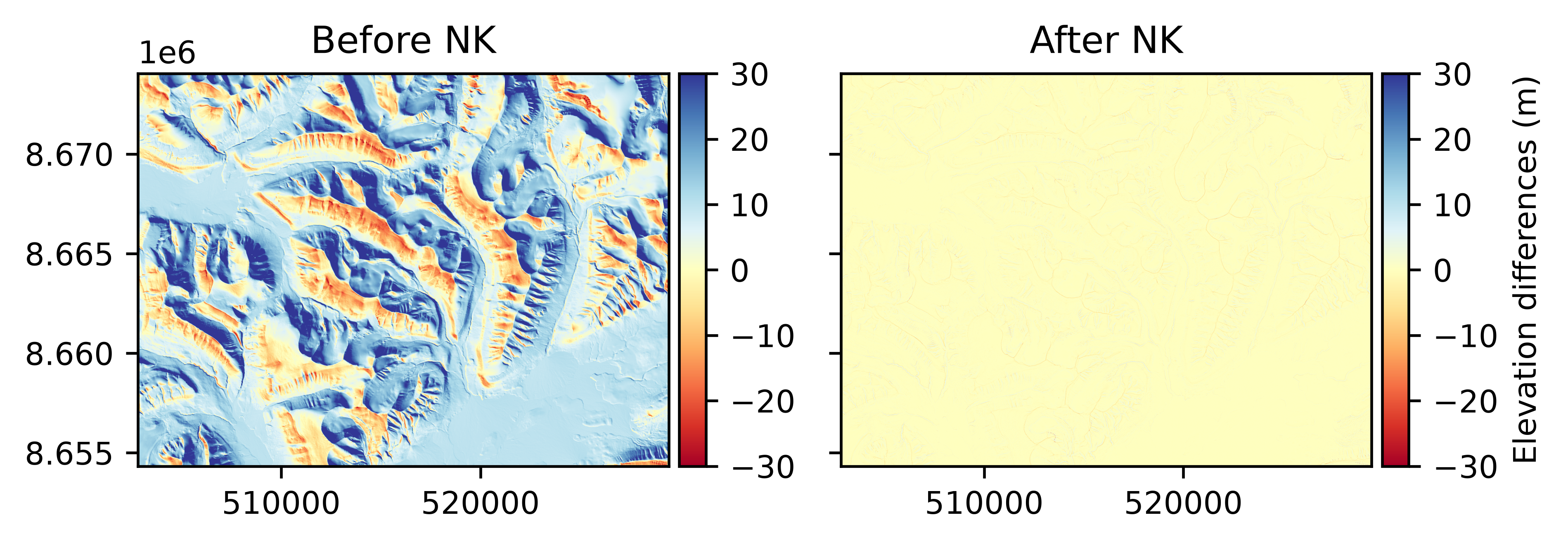
Nuth and Kääb (2011)

xdem.coreg.NuthKaab

• Performs: Horizontal and vertical shifts.

• Supports weights: Planned.

• Pros: Refines sub-pixel horizontal shifts accurately, with fast convergence.

• Cons: Diverges on flat terrain, as landforms are required to constrain the fit with aspect and slope.

The Nuth and Kääb (2011) coregistration approach estimates a horizontal translation iteratively by solving a cosine equation between the terrain slope, aspect and the elevation differences. The iteration stops if it reaches the maximum number of iteration limit, or if the iterative shift amplitude falls below a specified tolerance.

Show the code for adding a horizontal and vertical shift

Hide the code for adding a horizontal and vertical shift

x_shift = 30
y_shift = 30
z_shift = 10
# Affine matrix for 3D transformation
matrix = np.array(
    [
        [1, 0, 0, x_shift],
        [0, 1, 0, y_shift],
        [0, 0, 1, z_shift],
        [0, 0, 0, 1],
    ]
)
# We create misaligned elevation data
tba_dem_shifted = xdem.coreg.apply_matrix(ref_dem, matrix)

# Define a coregistration based on the Nuth and Kääb (2011) method
nuth_kaab = xdem.coreg.NuthKaab()
# Fit to data and apply
aligned_dem = nuth_kaab.fit_and_apply(ref_dem, tba_dem_shifted)

Show plotting code

Hide plotting code

# Plot before and after
f, ax = plt.subplots(1, 2)
ax[0].set_title("Before NK")
(tba_dem_shifted - ref_dem).plot(cmap='RdYlBu', vmin=-30, vmax=30, ax=ax[0])
ax[1].set_title("After NK")
(aligned_dem - ref_dem).plot(cmap='RdYlBu', vmin=-30, vmax=30, ax=ax[1], cbar_title="Elevation differences (m)")
_ = ax[1].set_yticklabels([])
plt.tight_layout()

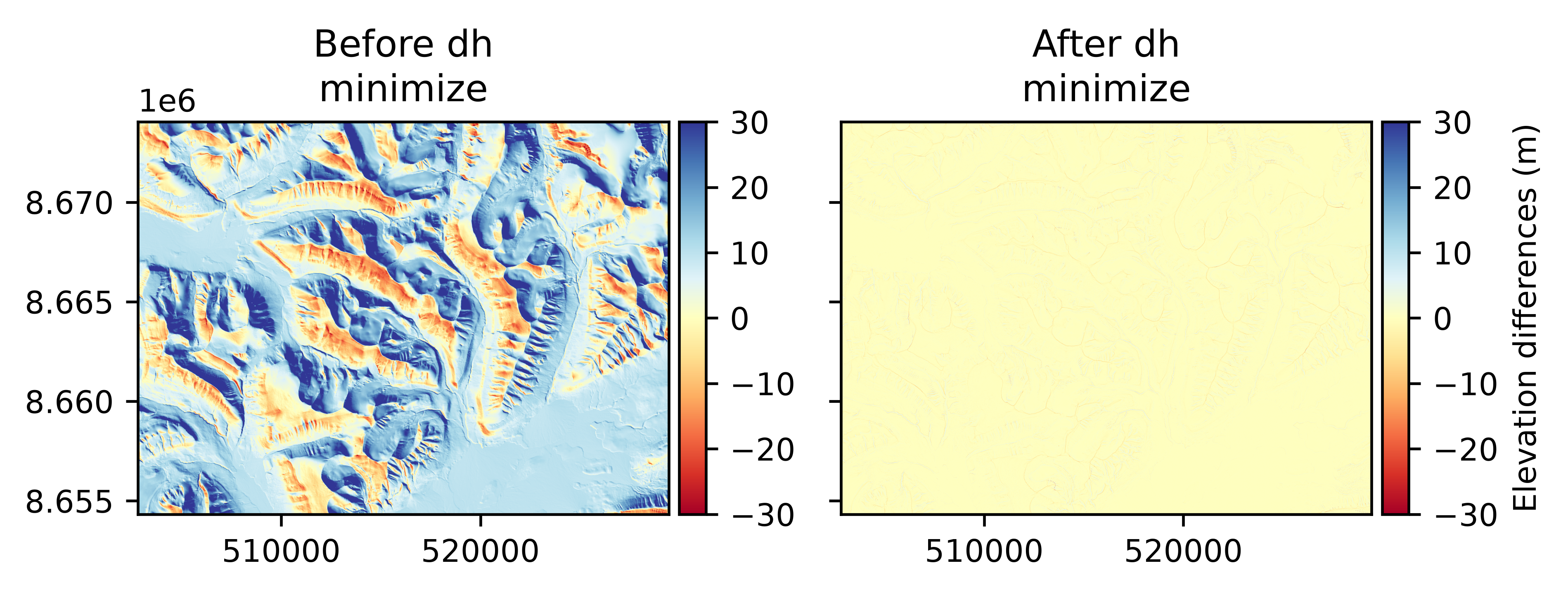
Minimization of dh

xdem.coreg.DhMinimize

• Performs: Horizontal and vertical shifts.

• Supports weights: Planned.

• Pros: Can be used to perform both local and global registration by tuning the minimizer.

• Cons: Sensitive to noise.

The minimization of elevation differences (or dh) coregistration approach estimates a horizontal translation by minimizing any statistic on the elevation differences, typically their spread (defaults to the NMAD).

# Define a coregistration based on the dh minimization approach
dh_minimize = xdem.coreg.DhMinimize()
# Fit to data and apply
aligned_dem = dh_minimize.fit_and_apply(ref_dem, tba_dem_shifted)

Show plotting code

Hide plotting code

# Plot before and after
f, ax = plt.subplots(1, 2)
ax[0].set_title("Before dh\nminimize")
(tba_dem_shifted - ref_dem).plot(cmap='RdYlBu', vmin=-30, vmax=30, ax=ax[0])
ax[1].set_title("After dh\nminimize")
(aligned_dem - ref_dem).plot(cmap='RdYlBu', vmin=-30, vmax=30, ax=ax[1], cbar_title="Elevation differences (m)")
_ = ax[1].set_yticklabels([])
plt.tight_layout()

Vertical shift

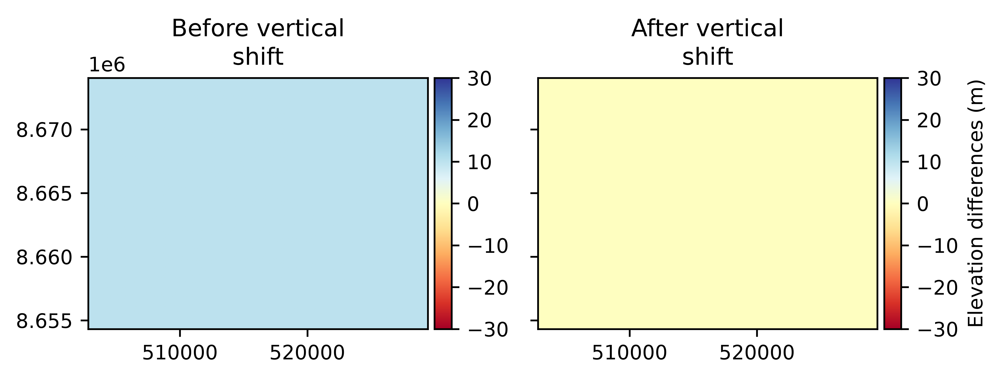
xdem.coreg.VerticalShift

Caution

Vertical shifting simply serves to refine a vertical translation over the entire elevation data. For transforming the 3D CRS, see the Vertical referencing feature page.

• Performs: Vertical translation based on central elevation differences estimated with any custom function (mean, median).

• Supports weights: Planned.

• Pros: Useful to have as independent step to refine vertical alignment precisely as it is the most sensitive to outliers, by refining inliers and the central estimate function.

• Cons: Always needs to be combined with another approach.

The vertical shift coregistration is simply a shift based on an estimate of the mean elevation differences with customizable arguments.

Show the code for adding a vertical shift

Hide the code for adding a vertical shift

# Apply a vertical shift of 10 meters
tba_dem_vshifted = ref_dem + 10

# Define a coregistration object based on a vertical shift correction
vshift = xdem.coreg.VerticalShift(vshift_reduc_func=np.median)
# Fit and apply
aligned_dem = vshift.fit_and_apply(ref_dem, tba_dem_vshifted)

Show plotting code

Hide plotting code

# Plot before and after
f, ax = plt.subplots(1, 2)
ax[0].set_title("Before vertical\nshift")
(tba_dem_vshifted - ref_dem).plot(cmap='RdYlBu', vmin=-30, vmax=30, ax=ax[0])
ax[1].set_title("After vertical\nshift")
(aligned_dem - ref_dem).plot(cmap='RdYlBu', vmin=-30, vmax=30, ax=ax[1], cbar_title="Elevation differences (m)")
_ = ax[1].set_yticklabels([])
plt.tight_layout()

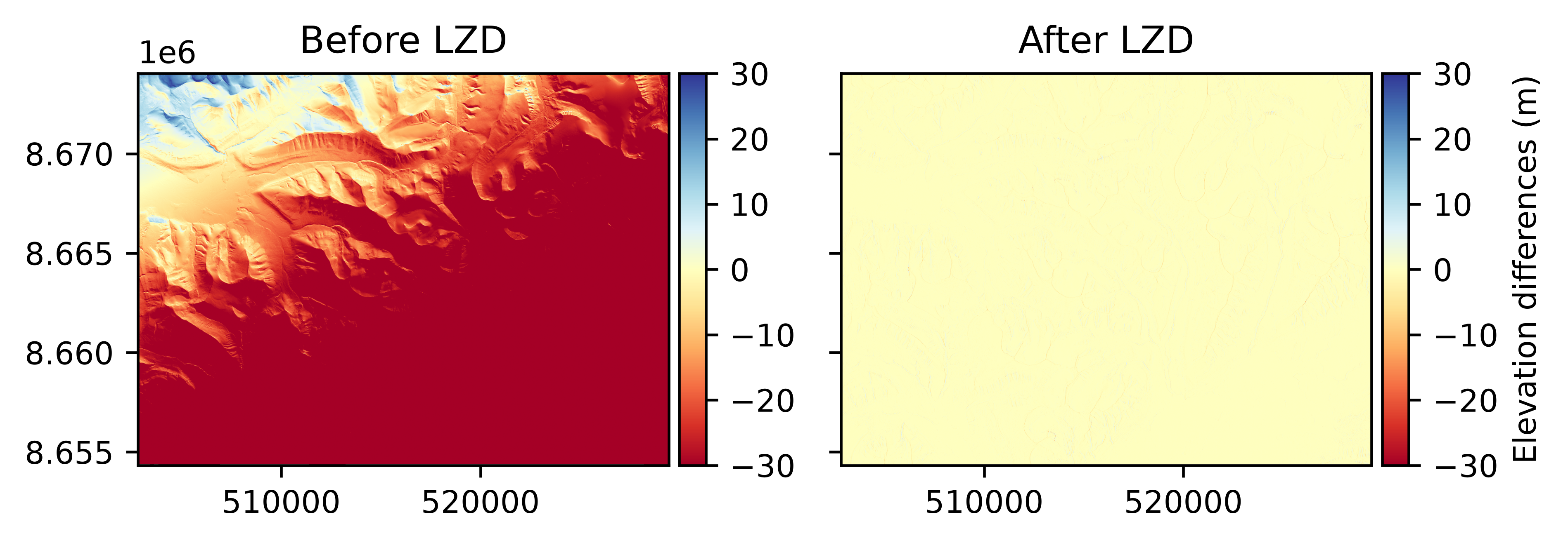
Least Z-difference

xdem.coreg.LZD

• Performs: Rigid transformation (3D translation + 3D rotation).

• Does not support weights.

• Pros: Good at solving sub-pixels shifts.

• Cons: Sensitive to elevation outliers.

Least Z-difference (LZD) coregistration is an iterative point-grid registration method from Rosenholm and Torlegård (1988).

Show the code for adding a shift and rotation

Hide the code for adding a shift and rotation

# Apply a rotation of 0.2 degrees in X, 0.1 in Y and 0 in Z
rotations = np.array([0.2, 0.1, 0])
# Add X/Y/Z shifts in meters
shifts = np.array([10, 20, 5])
# Affine matrix for 3D transformation
matrix = xdem.coreg.matrix_from_translations_rotations(*shifts, *rotations)

# We create misaligned elevation data
centroid = [ref_dem.bounds.left + 5000, ref_dem.bounds.top - 2000, np.median(ref_dem)]
tba_dem_shifted_rotated = xdem.coreg.apply_matrix(ref_dem, matrix, centroid=centroid)

# Define a coregistration based on LZD
lzd = xdem.coreg.LZD()
# Fit to data and apply
aligned_dem = lzd.fit_and_apply(ref_dem, tba_dem_shifted_rotated)

Show plotting code

Hide plotting code

# Plot before and after
f, ax = plt.subplots(1, 2)
ax[0].set_title("Before LZD")
(tba_dem_shifted_rotated - ref_dem).plot(cmap='RdYlBu', vmin=-30, vmax=30, ax=ax[0])
ax[1].set_title("After LZD")
(aligned_dem - ref_dem).plot(cmap='RdYlBu', vmin=-30, vmax=30, ax=ax[1], cbar_title="Elevation differences (m)")
_ = ax[1].set_yticklabels([])
plt.tight_layout()

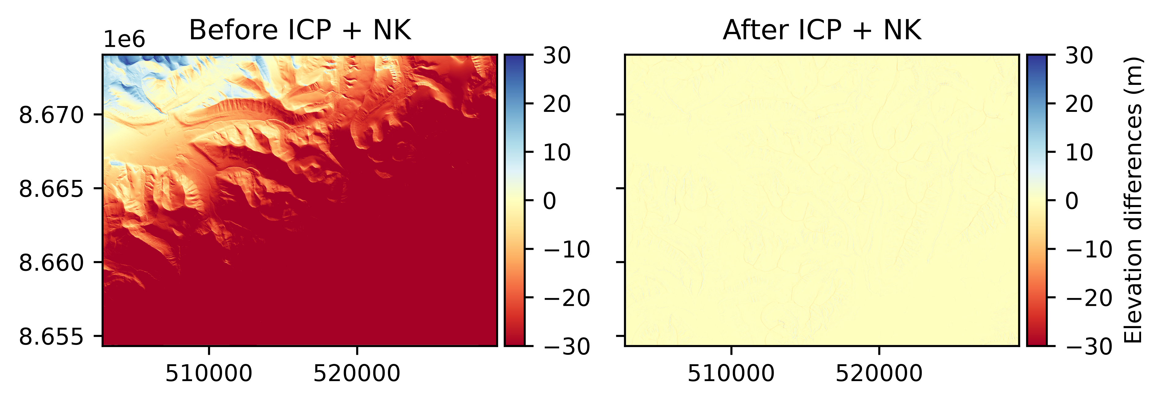
Iterative closest point

xdem.coreg.ICP

• Performs: Rigid transformation (3D translation + 3D rotation).

• Does not support weights.

• Pros: Efficient at estimating rotation and shifts simultaneously.

• Cons: Poor sub-pixel accuracy for horizontal shifts, sensitive to outliers, and runs slowly with large samples.

Iterative closest point (ICP) coregistration is an iterative point cloud registration method from Besl and McKay (1992) (point-to-point) or Chen and Medioni (1992) (point-to-plane). It aims at iteratively minimizing the distance between closest neighbours by applying sequential rigid transformations. For point-to-point, the 3D distance is used for the minimization while, for point-to-plane, the 3D distance projected on the plane normals is used instead. If DEMs are used as inputs, they are converted to point clouds. As for Nuth and Kääb (2011), the iteration stops if it reaches the maximum number of iteration limit or if the iterative transformation amplitude falls below a specified tolerance.

# Define a coregistration based on ICP
icp = xdem.coreg.ICP()
# Fit to data and apply
aligned_dem = icp.fit_and_apply(ref_dem, tba_dem_shifted_rotated)

Show plotting code

Hide plotting code

# Plot before and after
f, ax = plt.subplots(1, 2)
ax[0].set_title("Before ICP")
(tba_dem_shifted_rotated - ref_dem).plot(cmap='RdYlBu', vmin=-30, vmax=30, ax=ax[0])
ax[1].set_title("After ICP")
(aligned_dem - ref_dem).plot(cmap='RdYlBu', vmin=-30, vmax=30, ax=ax[1], cbar_title="Elevation differences (m)")
_ = ax[1].set_yticklabels([])
plt.tight_layout()

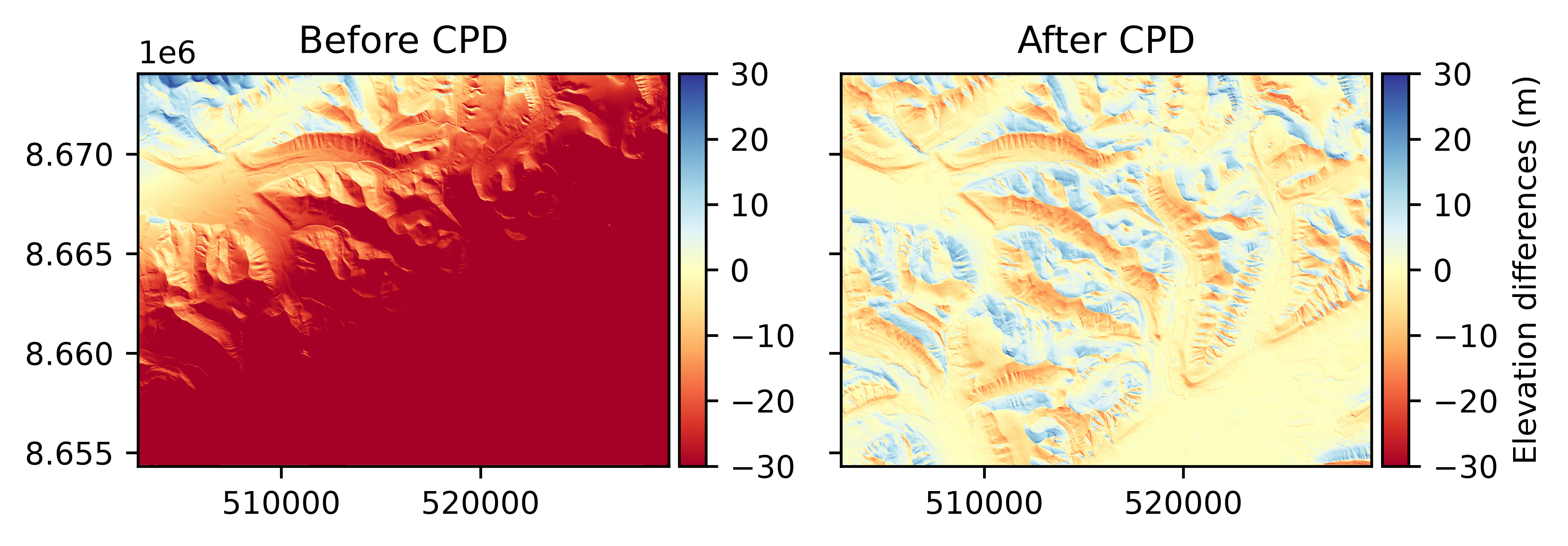
Coherent point drift

xdem.coreg.CPD

• Performs: Rigid transformation (3D translation + 3D rotation).

• Does not support weights.

• Pros: Needs fewer samples to work efficiently.

• Cons: Has trouble solving for horizontal translations if X/Y scale differs from Z scale, as GMM variance is the same in all dimensions.

Coherent point drift (CPD) coregistration is an iterative point cloud registration method from Myronenko and Song (2010). It is a probabilistic approach, iteratively fitting Gaussian mixture model (GMM) centroids for the reference point cloud on the target point cloud by maximizing the likelihood of the probability density estimation problem.

# Define a coregistration based on CPD
cpd = xdem.coreg.CPD()
# Fit to data and apply
aligned_dem = cpd.fit_and_apply(ref_dem, tba_dem_shifted_rotated)

Show plotting code

Hide plotting code

# Plot before and after
f, ax = plt.subplots(1, 2)
ax[0].set_title("Before CPD")
(tba_dem_shifted_rotated - ref_dem).plot(cmap='RdYlBu', vmin=-30, vmax=30, ax=ax[0])
ax[1].set_title("After CPD")
(aligned_dem - ref_dem).plot(cmap='RdYlBu', vmin=-30, vmax=30, ax=ax[1], cbar_title="Elevation differences (m)")
_ = ax[1].set_yticklabels([])
plt.tight_layout()

Building coregistration pipelines

The CoregPipeline object

Often, more than one coregistration approach is necessary to obtain the best results, and several need to be combined sequentially. A CoregPipeline can be constructed for this:

# We can list sequential coregistration methods to apply
pipeline = xdem.coreg.CoregPipeline([xdem.coreg.ICP(), xdem.coreg.NuthKaab()])

# Or sum them, which works identically as the syntax above
pipeline = xdem.coreg.ICP() + xdem.coreg.NuthKaab()

The CoregPipeline object exposes the same interface as the Coreg object. The results of a pipeline can be used in other programs by exporting the combined transformation matrix using to_matrix().

²Here again, this class is heavily inspired by SciKit-Learn’s Pipeline and make_pipeline() functionalities.

# Fit to data and apply the pipeline of ICP + Nuth and Kääb
aligned_dem = pipeline.fit_and_apply(ref_dem, tba_dem_shifted_rotated)

Show plotting code

Hide plotting code

# Plot before and after
f, ax = plt.subplots(1, 2)
ax[0].set_title("Before ICP + NK")
(tba_dem_shifted_rotated - ref_dem).plot(cmap='RdYlBu', vmin=-30, vmax=30, ax=ax[0])
ax[1].set_title("After ICP + NK")
(aligned_dem - ref_dem).plot(cmap='RdYlBu', vmin=-30, vmax=30, ax=ax[1], cbar_title="Elevation differences (m)")
_ = ax[1].set_yticklabels([])
plt.tight_layout()

Recommended pipelines

To ensure sub-pixel accuracy, the Nuth and Kääb (2011) coregistration should almost always be used as a final step. The approach does not account for rotations in the dataset, however, so a combination is often necessary. For small rotations, a 1st degree deramp can be used in combination:

pipeline = xdem.coreg.NuthKaab() + xdem.coreg.Deramp(poly_order=1)

For larger rotations, ICP can be used instead:

pipeline = xdem.coreg.ICP() + xdem.coreg.NuthKaab()

Additionally, ICP tends to fail with large initial vertical differences, so a preliminary vertical shifting can be used:

pipeline = xdem.coreg.VerticalShift() + xdem.coreg.ICP() + xdem.coreg.NuthKaab()

Coregistration metadata

The metadata surrounding a coregistration method, which can be displayed by info(), is stored in the meta nested dictionary. This metadata is divided into inputs and outputs. Input metadata corresponds to what arguments are used when initializing a Coreg object, while output metadata are created during the call to fit(). Together, they allow to apply the transformation during the apply() step of the coregistration.

# Example of metadata info after fitting
my_coreg_pipeline.info()

Generic coregistration information 
  Method:       NuthKaab 
  Is affine?    True 
  Fit called?   True 
Inputs
  Randomization
    Subsample size requested:                     500000.0
    Random generator:                             None
  Fitting and binning
    Fit, bin or bin+fit:                          bin_and_fit
    Function to fit:                              _nuth_kaab_fit_func
    Optimizer for fitting:                        curve_fit
    Bin sizes or edges:                           72
    Binning statistic:                            nanmedian
    Number of dimensions of binning and fitting:  1
    Names of bias variables:                      ['aspect']
  Affine
    Vertical shift activated:                     True
  Iterative
    Maximum number of iterations:                 10
    Tolerance to reach (pixel size):              0.001
Outputs
  Randomization
    Subsample size drawn from valid values:       500000
  Affine
    Eastward shift estimated (georeferenced unit):8.55
    Northward shift estimated (georeferenced unit):1.28
    Vertical shift estimated (elevation unit):    -2.43

For both inputs and outputs, four consistent categories of metadata are defined.

Note: Some metadata, such as the parameters fit_or_bin and fit_func described below, are pre-defined for affine coregistration methods and cannot be modified. They only take user-specified value for Bias correction.

1. Randomization metadata (common to all):

• An input subsample to define the subsample size of valid data to use in all methods (recommended for performance),

• An input random_state to define the random seed for reproducibility of the subsampling (and potentially other random aspects such as optimizers),

• An output subsample_final that stores the final subsample size used, which can be smaller than requested depending on the amount of valid data intersecting the two elevation datasets.

2. Fitting and binning metadata (common to nearly all methods):

• An input fit_or_bin to either fit a parametric model by passing “fit”, perform an empirical binning by passing “bin”, or to fit a parametric model to the binning with “bin_and_fit” (only “fit” or “bin_and_fit” possible for affine methods),

• An input fit_func to pass any parametric function to fit to the bias (pre-defined for affine methods),

• An input fit_optimizer to pass any optimizer function to perform the fit minimization,

• An input bin_sizes to pass the size or edges of the bins for each variable,

• An input bin_statistic to pass the statistic to compute in each bin,

• An input bin_apply_method to pass the method to apply the binning for correction,

• An output fit_params that stores the optimized parameters for fit_func,

• An output fit_perr that stores the error of optimized parameters (only for default fit_optimizer),

• An output bin_dataframe that stores the dataframe of binned statistics.

3. Iteration metadata (common to all iterative methods):

• An input max_iterations to define the maximum number of iterations at which to stop the method,

• An input tolerance to define the tolerance at which to stop iterations (tolerance unit defined in method description),

• An output last_iteration that stores the last iteration of the method,

• An output all_tolerances that stores the tolerances computed at each iteration.

4. Affine metadata (common to all affine methods):

• An input only_translation to define if a coregistration should solve only for translations instead of a full rigid transformation (translations and rotations),

• An input standardize to define if the input data should be standardized to the unit sphere before coregistration (to improve numerical convergence),

• An input initial_shift that defines the estimated initial x and y shifts in georeferenced units, applied before fit step.

• An output matrix that stores the estimated affine matrix,

• An output centroid that stores the centroid coordinates with which to apply the affine transformation,

• Outputs shift_x, shift_y and shift_z that store the easting, northing and vertical offsets, respectively.

Tip

In xDEM, you can extract the translations and rotations of an affine matrix using xdem.coreg.AffineCoreg.to_translations and xdem.coreg.AffineCoreg.to_rotations.

To further manipulate affine matrices, see the documentation of pytransform3d.

5. Specific metadata (only for certain methods):

These metadata are only inputs specific to a given method, outlined in the method description.

For instance, for xdem.coreg.Deramp, an input poly_order to define the polynomial order used for the fit, and for xdem.coreg.DirectionalBias, an input angle to define the angle at which to do the directional correction.

Dividing coregistration in blocks

The BlockwiseCoreg object

Caution

The BlockwiseCoreg feature is still experimental. Currently, it is only tested for the affine coregistration methods and for translation only. Rotation shifts will be soon implemented, but not yet available. Please set only_translation=True when initializing the coregistration method ICP(), LZD() or CPD().

A BlockwiseCoreg splits DEMs into grids, then the selected coregistration method runs independently in each block. After this step, the results are combined (using interpolation or soon aggregation) to obtain the overall offset. The first advantage is improved detection of local errors. The second is that, by default, blocks are loaded sequentially, which helps reduce memory usage. As a result, it is possible to work with larger datasets.

Note

The block_size_fit parameter adjusts the size of the tiles over which the coregistration methods are computed. The block_size_apply parameter allows the DEM to be aligned in blocks to optimize memory usage. Smaller blocks during the apply step reduce memory usage but increase computing time. These two parameters do not need to be the same size.

In this example, processing is performed sequentially. However, it is possible to enable multiprocessing on BlockwiseCoreg, the configuration is described in Blockwise coregistration example.

blockwise = xdem.coreg.BlockwiseCoreg(xdem.coreg.NuthKaab(),
                                      block_size_fit=500,
                                      block_size_apply=500,
                                      parent_path="")
blockwise.fit(ref_dem, tba_dem_shifted)

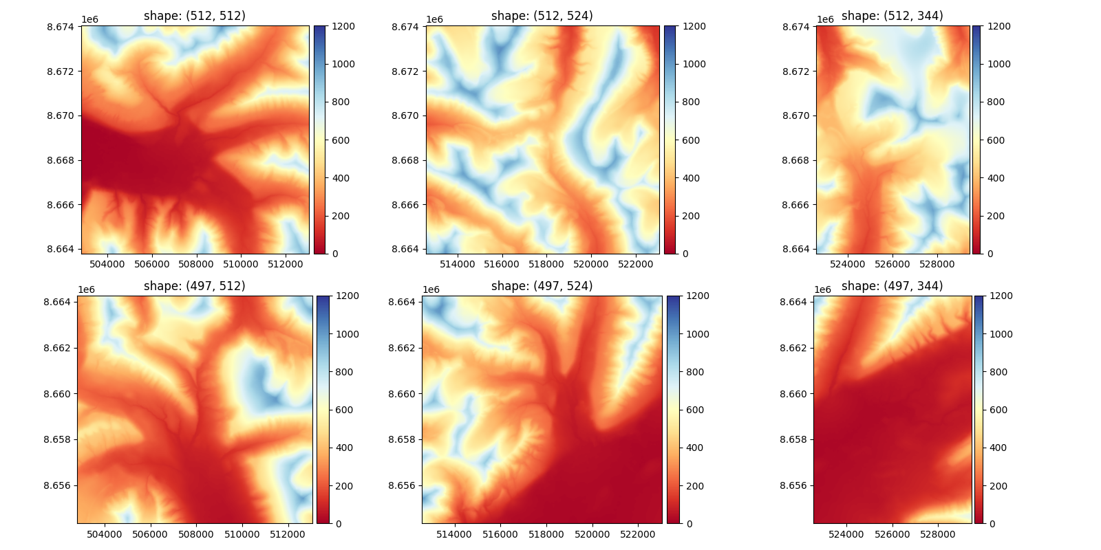
To better visualize the blocks, here is how fit(), divides a DEM with a block_size_fit of 500.

The results of each tile coregistration are saved in the meta parameters, they will be used to estimate the overall offset.

blockwise.meta

{'inputs': {'random': {'subsample': 500000.0},
  'fitorbin': {'fit_or_bin': 'bin_and_fit',
   'fit_func': <function xdem.coreg.affine._nuth_kaab_fit_func(xx: 'NDArrayf', *params: 'tuple[float, float, float]') -> 'NDArrayf'>,
   'fit_optimizer': <function scipy.optimize._minpack_py.curve_fit(f, xdata, ydata, p0=None, sigma=None, absolute_sigma=False, check_finite=None, bounds=(-inf, inf), method=None, jac=None, *, full_output=False, nan_policy=None, **kwargs)>,
   'bin_sizes': 72,
   'bin_statistic': <function nanmedian at 0x70e23c226f70>},
  'iterative': {'max_iterations': 10, 'tolerance': 0.001},
  'specific': {},
  'affine': {'apply_vshift': True}},
 'outputs': {'0_0': {'shift_x': np.float64(-29.981913351133795),
   'shift_y': np.float64(-30.027430562505327),
   'shift_z': -9.986330953243481},
  '0_1': {'shift_x': np.float64(-29.979588607929703),
   'shift_y': np.float64(-30.10763482845488),
   'shift_z': -10.025389258707946},
  '0_2': {'shift_x': np.float64(-29.979768781352355),
   'shift_y': np.float64(-30.109483370434397),
   'shift_z': -10.010137734460159},
  '1_0': {'shift_x': np.float64(-29.974009429630023),
   'shift_y': np.float64(-30.05259989072575),
   'shift_z': -9.99987599765651},
  '1_1': {'shift_x': np.float64(-30.00567713394534),
   'shift_y': np.float64(-30.093419769258972),
   'shift_z': -9.998554982277906},
  '1_2': {'shift_x': np.float64(-29.97445999169496),
   'shift_y': np.float64(-30.041518430878373),
   'shift_z': -9.989712006770727}}}

Once this first step has been completed, you can proceed to the apply() step. At this step, an interpolation method will be used to estimate the overall offset. The result obtained is then applied to the entire DEM, also by blocks, but this time with an overlap to avoid edge effects. This overlap corresponds to the maximum offset obtained during the fit().

aligned_dem = blockwise.apply(tba_dem_shifted)

Here are the blocks for the apply(), but this time with the overlap.

Show plotting code

Hide plotting code

# Plot before and after
f, ax = plt.subplots(1, 2)
ax[0].set_title("Before block NK")
(tba_dem_shifted - ref_dem).plot(cmap='RdYlBu', vmin=-30, vmax=30, ax=ax[0])
ax[1].set_title("After block NK")
(aligned_dem - ref_dem).plot(cmap='RdYlBu', vmin=-30, vmax=30, ax=ax[1], cbar_title="Elevation differences (m)")
_ = ax[1].set_yticklabels([])