Normalized regional hypsometric interpolation

There are many ways of interpolating gaps in a dDEM. In the case of glaciers, one very useful fact is that elevation change generally varies with elevation. This means that if valid pixels exist in a certain elevation bin, their values can be used to fill other pixels in the same approximate elevation. Filling gaps by elevation is the main basis of “hypsometric interpolation approaches”, of which there are many variations of.

One problem with simple hypsometric approaches is that they may not work for glaciers with different elevation ranges and scales. Let’s say we have two glaciers: one gigantic reaching from 0-1000 m, and one small from 900-1100 m. Usually in the 2000s, glaciers thin rapidly at the bottom, while they may be neutral or only thin slightly in the top. If we extrapolate the hypsometric signal of the gigantic glacier to use on the small one, it may seem like the smaller glacier has almost no change whatsoever. This may be right, or it may be catastrophically wrong!

Normalized regional hypsometric interpolation solves the scale and elevation range problems in one go. It:

1. Calculates a regional signal using the weighted average of each glacier’s normalized signal:

   1. The glacier’s elevation range is scaled from 0-1 to be elevation-independent.

   2. The glaciers elevation change is scaled from 0-1 to be magnitude-independent.

   3. A weight is assigned by the amount of valid pixels (well-covered large glaciers gain a higher weight)

2. Re-scales that signal to fit each glacier once determined.

The consequence is a much more accurate interpolation approach that can be used in a multitude of glacierized settings.

import geoutils as gu

import matplotlib.pyplot as plt
import numpy as np

import xdem
import xdem.misc

Example files

dem_2009 = xdem.DEM(xdem.examples.get_path("longyearbyen_ref_dem"))
dem_1990 = xdem.DEM(xdem.examples.get_path("longyearbyen_tba_dem_coreg"))

glacier_outlines = gu.Vector(xdem.examples.get_path("longyearbyen_glacier_outlines"))

# Rasterize the glacier outlines to create an index map.
# Stable ground is 0, the first glacier is 1, the second is 2, etc.
glacier_index_map = glacier_outlines.rasterize(dem_2009)

plt_extent = [
    dem_2009.bounds.left,
    dem_2009.bounds.right,
    dem_2009.bounds.bottom,
    dem_2009.bounds.top,
]

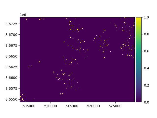
To test the method, we can generate a semi-random mask to assign nans to glacierized areas. Let’s remove 30% of the data.

np.random.seed(42)
random_nans = (xdem.misc.generate_random_field(dem_1990.shape, corr_size=5) > 0.7) & (glacier_index_map > 0)

random_nans.plot()

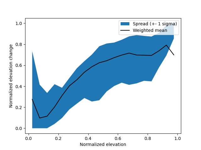
The normalized hypsometric signal shows the tendency for elevation change as a function of elevation. The magnitude may vary between glaciers, but the shape is generally similar. Normalizing by both elevation and elevation change, and then re-scaling the signal to every glacier, ensures that it is as accurate as possible. NOTE: The hypsometric signal does not need to be generated separately; it will be created by xdem.volume.norm_regional_hypsometric_interpolation(). Generating it first, however, allows us to visualize and validate it.

ddem = dem_2009 - dem_1990
ddem_voided = np.where(random_nans.data, np.nan, ddem.data)

signal = xdem.volume.get_regional_hypsometric_signal(
    ddem=ddem_voided,
    ref_dem=dem_2009.data,
    glacier_index_map=glacier_index_map,
)

plt.fill_between(signal.index.mid, signal["sigma-1-lower"], signal["sigma-1-upper"], label="Spread (+- 1 sigma)")
plt.plot(signal.index.mid, signal["w_mean"], color="black", label="Weighted mean")
plt.ylabel("Normalized elevation change")
plt.xlabel("Normalized elevation")
plt.legend()
plt.show()

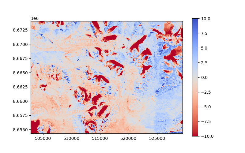
The signal can now be used (or simply estimated again if not provided) to interpolate the DEM.

ddem_filled = xdem.volume.norm_regional_hypsometric_interpolation(
    voided_ddem=ddem_voided, ref_dem=dem_2009, glacier_index_map=glacier_index_map, regional_signal=signal
)


plt.figure(figsize=(8, 5))
plt.imshow(ddem_filled.data, cmap="coolwarm_r", vmin=-10, vmax=10, extent=plt_extent)
plt.colorbar()
plt.show()

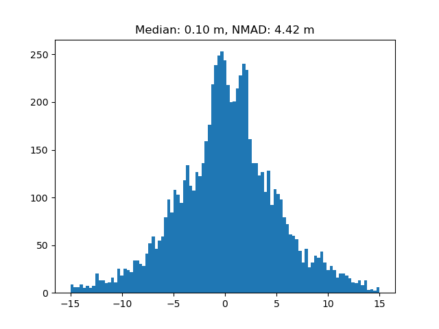
We can plot the difference between the actual and the interpolated values, to validate the method.

difference = (ddem_filled - ddem)[random_nans]
median = np.nanmedian(difference)
nmad = xdem.spatialstats.nmad(difference)

plt.title(f"Median: {median:.2f} m, NMAD: {nmad:.2f} m")
plt.hist(difference.data, bins=np.linspace(-15, 15, 100))
plt.show()

/home/docs/checkouts/readthedocs.org/user_builds/xdem/conda/latest/lib/python3.11/site-packages/numpy/core/fromnumeric.py:771: UserWarning: Warning: 'partition' will ignore the 'mask' of the MaskedArray.
  a.partition(kth, axis=axis, kind=kind, order=order)

As we see, the median is close to zero, while the NMAD varies slightly more. This is expected, as the regional signal is good for multiple glaciers at once, but it cannot account for difficult local topography and meteorological conditions. It is therefore highly recommended for large regions; just don’t zoom in too close!