Spatial propagation of elevation errors

Propagating elevation errors spatially accounting for heteroscedasticity and spatial correlation is complex. It requires computing the pairwise correlations between all points of an area of interest (be it for a sum, mean, or other operation), which is computationally intensive. Here, we rely on published formulations to perform computationally-efficient spatial propagation for the mean of elevation (or elevation differences) in an area.

References: Hugonnet et al. (2022), Figure S16, Equations 17–19 and Rolstad et al. (2009), Equation 8.

import geoutils as gu
import matplotlib.pyplot as plt

import numpy as np

import xdem

We load the same data, and perform the same calculations on heteroscedasticity and spatial correlations of errors as in the Elevation error map and Spatial correlation of errors examples.

dh = xdem.DEM(xdem.examples.get_path("longyearbyen_ddem"))
ref_dem = xdem.DEM(xdem.examples.get_path("longyearbyen_ref_dem"))
glacier_outlines = gu.Vector(xdem.examples.get_path("longyearbyen_glacier_outlines"))
slope, maximum_curvature = xdem.terrain.get_terrain_attribute(ref_dem, attribute=["slope", "maximum_curvature"])
errors, df_binning, error_function = xdem.spatialstats.infer_heteroscedasticity_from_stable(
    dvalues=dh, list_var=[slope, maximum_curvature], list_var_names=["slope", "maxc"], unstable_mask=glacier_outlines
)

We use the error map to standardize the elevation differences before variogram estimation, following Equation 12 of Hugonnet et al. (2022), which is more robust as it removes the variance variability due to heteroscedasticity.

zscores = dh / errors
emp_variogram, params_variogram_model, spatial_corr_function = xdem.spatialstats.infer_spatial_correlation_from_stable(
    dvalues=zscores, list_models=["Gaussian", "Spherical"], unstable_mask=glacier_outlines, random_state=42
)

With our estimated heteroscedasticity and spatial correlation, we can now perform the spatial propagation of errors. We select two glaciers intersecting this elevation change map in Svalbard. The best estimation of their standard error is done by directly providing the shapefile, which relies on Equation 18 of Hugonnet et al. (2022).

areas = [
    glacier_outlines.ds[glacier_outlines.ds["NAME"] == "Brombreen"],
    glacier_outlines.ds[glacier_outlines.ds["NAME"] == "Medalsbreen"],
]
stderr_glaciers = xdem.spatialstats.spatial_error_propagation(
    areas=areas, errors=errors, params_variogram_model=params_variogram_model
)

for glacier_name, stderr_gla in [("Brombreen", stderr_glaciers[0]), ("Medalsbreen", stderr_glaciers[1])]:
    print(f"The error (1-sigma) in mean elevation change for {glacier_name} is {stderr_gla:.2f} meters.")

The error (1-sigma) in mean elevation change for Brombreen is 0.81 meters.
The error (1-sigma) in mean elevation change for Medalsbreen is 0.88 meters.

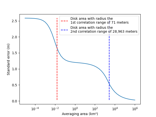
When passing a numerical area value, we compute an approximation with disk shape from Equation 8 of Rolstad et al. (2009). This approximation is practical to visualize changes in elevation error when averaging over different area sizes, but is less accurate to estimate the standard error of a certain area shape.

areas = 10 ** np.linspace(1, 12)
stderrs = xdem.spatialstats.spatial_error_propagation(
    areas=areas, errors=errors, params_variogram_model=params_variogram_model
)
plt.plot(areas / 10**6, stderrs)
plt.xlabel("Averaging area (km²)")
plt.ylabel("Standard error (m)")
plt.vlines(
    x=np.pi * params_variogram_model["range"].values[0] ** 2 / 10**6,
    ymin=np.min(stderrs),
    ymax=np.max(stderrs),
    colors="red",
    linestyles="dashed",
    label="Disk area with radius the\n1st correlation range of {:,.0f} meters".format(
        params_variogram_model["range"].values[0]
    ),
)
plt.vlines(
    x=np.pi * params_variogram_model["range"].values[1] ** 2 / 10**6,
    ymin=np.min(stderrs),
    ymax=np.max(stderrs),
    colors="blue",
    linestyles="dashed",
    label="Disk area with radius the\n2nd correlation range of {:,.0f} meters".format(
        params_variogram_model["range"].values[1]
    ),
)
plt.xscale("log")
plt.legend()
plt.show()