Standardization for stable terrain as error proxy

Digital elevation models have both a precision that can vary with terrain or instrument-related variables, and a spatial correlation of errors that can be due to effects of resolution, processing or instrument noise. Accouting for non-stationarities in elevation errors is essential to use stable terrain as a proxy to infer the precision on other types of terrain and reliably use spatial statistics (see spatialstats).

Here, we show an example of standardization of the data based on terrain-dependent explanatory variables (see Elevation error map) and combine it with an analysis of spatial correlation (see Spatial correlation of errors) .

Reference: Hugonnet et al. (2022), Equation 12.

import geoutils as gu

import matplotlib.pyplot as plt
import numpy as np

import xdem
from xdem.spatialstats import nmad

We start by estimating the elevation heteroscedasticity and deriving a terrain-dependent measurement error as a function of both slope and maximum curvature, as shown in the Elevation error map example.

# Load the data
ref_dem = xdem.DEM(xdem.examples.get_path("longyearbyen_ref_dem"))
dh = xdem.DEM(xdem.examples.get_path("longyearbyen_ddem"))
glacier_outlines = gu.Vector(xdem.examples.get_path("longyearbyen_glacier_outlines"))
mask_glacier = glacier_outlines.create_mask(dh)

# Compute the slope and maximum curvature
slope, planc, profc = xdem.terrain.get_terrain_attribute(
    dem=ref_dem, attribute=["slope", "planform_curvature", "profile_curvature"]
)

# Remove values on unstable terrain
dh_arr = dh[~mask_glacier].filled(np.nan)
slope_arr = slope[~mask_glacier].filled(np.nan)
planc_arr = planc[~mask_glacier].filled(np.nan)
profc_arr = profc[~mask_glacier].filled(np.nan)
maxc_arr = np.maximum(np.abs(planc_arr), np.abs(profc_arr))

# Remove large outliers
dh_arr[np.abs(dh_arr) > 4 * xdem.spatialstats.nmad(dh_arr)] = np.nan

# Define bins for 2D binning
custom_bin_slope = np.unique(
    np.concatenate(
        [
            np.nanquantile(slope_arr, np.linspace(0, 0.95, 20)),
            np.nanquantile(slope_arr, np.linspace(0.96, 0.99, 5)),
            np.nanquantile(slope_arr, np.linspace(0.991, 1, 10)),
        ]
    )
)

custom_bin_curvature = np.unique(
    np.concatenate(
        [
            np.nanquantile(maxc_arr, np.linspace(0, 0.95, 20)),
            np.nanquantile(maxc_arr, np.linspace(0.96, 0.99, 5)),
            np.nanquantile(maxc_arr, np.linspace(0.991, 1, 10)),
        ]
    )
)

# Perform 2D binning to estimate the measurement error with slope and maximum curvature
df = xdem.spatialstats.nd_binning(
    values=dh_arr,
    list_var=[slope_arr, maxc_arr],
    list_var_names=["slope", "maxc"],
    statistics=["count", np.nanmedian, nmad],
    list_var_bins=[custom_bin_slope, custom_bin_curvature],
)

# Estimate an interpolant of the measurement error with slope and maximum curvature
slope_curv_to_dh_err = xdem.spatialstats.interp_nd_binning(
    df, list_var_names=["slope", "maxc"], statistic="nmad", min_count=30
)
maxc = np.maximum(np.abs(profc), np.abs(planc))

# Estimate a measurement error per pixel
dh_err = slope_curv_to_dh_err((slope.data, maxc.data))

Using the measurement error estimated for each pixel, we standardize the elevation differences by applying a simple division:

z_dh = dh.data / dh_err

We remove values on glacierized terrain and large outliers.

z_dh.data[mask_glacier.data] = np.nan
z_dh.data[np.abs(z_dh.data) > 4] = np.nan

We perform a scale-correction for the standardization, to ensure that the spread of the data is exactly 1. The NMAD is used as a robust measure for the spread (see Dispersion).

print(f"NMAD before scale-correction: {nmad(z_dh.data):.1f}")
scale_fac_std = nmad(z_dh.data)
z_dh = z_dh / scale_fac_std
print(f"NMAD after scale-correction: {nmad(z_dh.data):.1f}")

plt.figure(figsize=(8, 5))
plt_extent = [
    ref_dem.bounds.left,
    ref_dem.bounds.right,
    ref_dem.bounds.bottom,
    ref_dem.bounds.top,
]
ax = plt.gca()
glacier_outlines.ds.plot(ax=ax, fc="none", ec="tab:gray")
ax.plot([], [], color="tab:gray", label="Glacier 1990 outlines")
plt.imshow(z_dh.squeeze(), cmap="RdYlBu", vmin=-3, vmax=3, extent=plt_extent)
cbar = plt.colorbar()
cbar.set_label("Standardized elevation differences (m)")
plt.legend(loc="lower right")
plt.show()

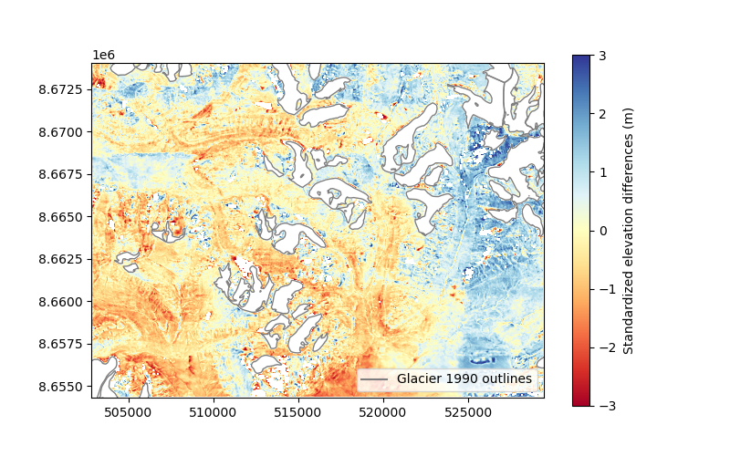
NMAD before scale-correction: 1.0
NMAD after scale-correction: 1.0

Now, we can perform an analysis of spatial correlation as shown in the Estimation and modelling of spatial variograms example, by estimating a variogram and fitting a sum of two models. Dowd’s variogram is used for robustness in conjunction with the NMAD (see Measures of spatial autocorrelation).

df_vgm = xdem.spatialstats.sample_empirical_variogram(
    values=z_dh.data.squeeze(),
    gsd=dh.res[0],
    subsample=1000,
    n_variograms=10,
    estimator="dowd",
    random_state=42,
)

func_sum_vgm, params_vgm = xdem.spatialstats.fit_sum_model_variogram(
    ["Gaussian", "Spherical"], empirical_variogram=df_vgm
)
xdem.spatialstats.plot_variogram(
    df_vgm,
    xscale_range_split=[100, 1000, 10000],
    list_fit_fun=[func_sum_vgm],
    list_fit_fun_label=["Standardized double-range variogram"],
)

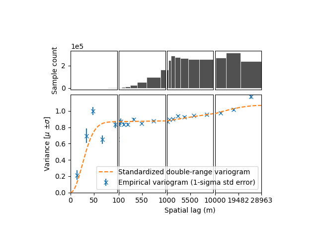
With standardized input, the variogram should converge towards one. With the input data close to a stationary variance, the variogram will be more robust as it won’t be affected by changes in variance due to terrain- or instrument-dependent variability of measurement error. The variogram should only capture changes in variance due to spatial correlation.

How to use this standardized spatial analysis to compute final uncertainties?

Let’s take the example of two glaciers of similar size: Svendsenbreen and Medalsbreen, which are respectively north and south-facing. The south-facing Medalsbreen glacier is subject to more sun exposure, and thus should be located in higher slopes, with possibly higher curvatures.

svendsen_shp = gu.Vector(glacier_outlines.ds[glacier_outlines.ds["NAME"] == "Svendsenbreen"])
svendsen_mask = svendsen_shp.create_mask(dh)

medals_shp = gu.Vector(glacier_outlines.ds[glacier_outlines.ds["NAME"] == "Medalsbreen"])
medals_mask = medals_shp.create_mask(dh)

plt.figure(figsize=(8, 5))
ax = plt.gca()
plt_extent = [
    ref_dem.bounds.left,
    ref_dem.bounds.right,
    ref_dem.bounds.bottom,
    ref_dem.bounds.top,
]
plt.imshow(slope.data, cmap="Blues", vmin=0, vmax=40, extent=plt_extent)
cbar = plt.colorbar(ax=ax)
cbar.set_label("Slope (degrees)")
svendsen_shp.ds.plot(ax=ax, fc="none", ec="tab:olive", lw=2)
medals_shp.ds.plot(ax=ax, fc="none", ec="tab:gray", lw=2)
plt.plot([], [], color="tab:olive", label="Medalsbreen")
plt.plot([], [], color="tab:gray", label="Svendsenbreen")
plt.legend(loc="lower left")
plt.show()

print(f"Average slope of Svendsenbreen glacier: {np.nanmean(slope[svendsen_mask]):.1f}")
print(f"Average maximum curvature of Svendsenbreen glacier: {np.nanmean(maxc[svendsen_mask]):.3f}")

print(f"Average slope of Medalsbreen glacier: {np.nanmean(slope[medals_mask]):.1f}")
print(f"Average maximum curvature of Medalsbreen glacier : {np.nanmean(maxc[medals_mask]):.1f}")

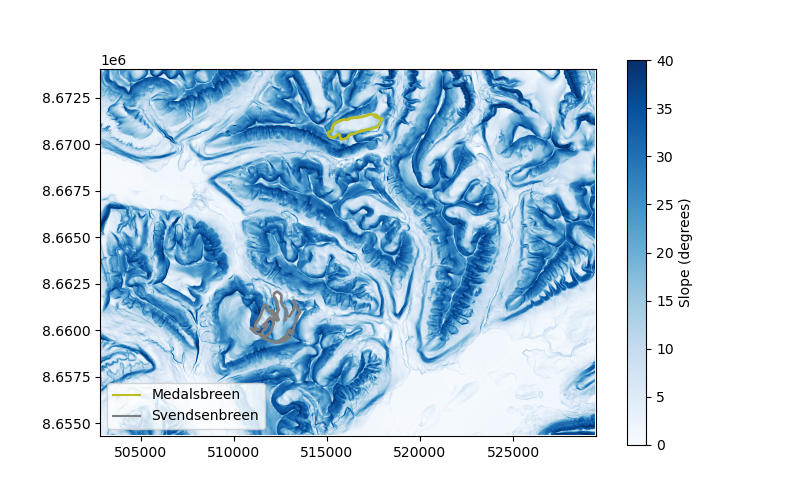
Average slope of Svendsenbreen glacier: 11.7
Average maximum curvature of Svendsenbreen glacier: 0.233
Average slope of Medalsbreen glacier: 18.5
Average maximum curvature of Medalsbreen glacier : 0.4

We calculate the number of effective samples for each glacier based on the variogram

svendsen_neff = xdem.spatialstats.neff_circular_approx_numerical(
    area=svendsen_shp.ds.area.values[0], params_variogram_model=params_vgm
)

medals_neff = xdem.spatialstats.neff_circular_approx_numerical(
    area=medals_shp.ds.area.values[0], params_variogram_model=params_vgm
)

print(f"Number of effective samples of Svendsenbreen glacier: {svendsen_neff:.1f}")
print(f"Number of effective samples of Medalsbreen glacier: {medals_neff:.1f}")

Number of effective samples of Svendsenbreen glacier: 4.4
Number of effective samples of Medalsbreen glacier: 4.4

Due to the long-range spatial correlations affecting the elevation differences, both glacier have a similar, low number of effective samples. This transcribes into a large standardized integrated error.

svendsen_z_err = 1 / np.sqrt(svendsen_neff)
medals_z_err = 1 / np.sqrt(medals_neff)

print(f"Standardized integrated error of Svendsenbreen glacier: {svendsen_z_err:.1f}")
print(f"Standardized integrated error of Medalsbreen glacier: {medals_z_err:.1f}")

Standardized integrated error of Svendsenbreen glacier: 0.5
Standardized integrated error of Medalsbreen glacier: 0.5

Finally, we destandardize the spatially integrated errors based on the measurement error dependent on slope and maximum curvature. This yields the uncertainty into the mean elevation change for each glacier.

# Destandardize the uncertainty
fac_svendsen_dh_err = scale_fac_std * np.nanmean(dh_err[svendsen_mask.data])
fac_medals_dh_err = scale_fac_std * np.nanmean(dh_err[medals_mask.data])
svendsen_dh_err = fac_svendsen_dh_err * svendsen_z_err
medals_dh_err = fac_medals_dh_err * medals_z_err

# Derive mean elevation change
svendsen_dh = np.nanmean(dh.data[svendsen_mask.data])
medals_dh = np.nanmean(dh.data[medals_mask.data])

# Plot the result
plt.figure(figsize=(8, 5))
ax = plt.gca()
plt.imshow(dh.data, cmap="RdYlBu", vmin=-50, vmax=50, extent=plt_extent)
cbar = plt.colorbar(ax=ax)
cbar.set_label("Elevation differences (m)")
svendsen_shp.ds.plot(ax=ax, fc="none", ec="tab:olive", lw=2)
medals_shp.ds.plot(ax=ax, fc="none", ec="tab:gray", lw=2)
plt.plot([], [], color="tab:olive", label="Svendsenbreen glacier")
plt.plot([], [], color="tab:gray", label="Medalsbreen glacier")
ax.text(
    svendsen_shp.ds.centroid.x.values[0],
    svendsen_shp.ds.centroid.y.values[0] - 1500,
    f"{svendsen_dh:.2f} \n$\\pm$ {svendsen_dh_err:.2f}",
    color="tab:olive",
    fontweight="bold",
    va="top",
    ha="center",
    fontsize=12,
)
ax.text(
    medals_shp.ds.centroid.x.values[0],
    medals_shp.ds.centroid.y.values[0] + 2000,
    f"{medals_dh:.2f} \n$\\pm$ {medals_dh_err:.2f}",
    color="tab:gray",
    fontweight="bold",
    va="bottom",
    ha="center",
    fontsize=12,
)
plt.legend(loc="lower left")
plt.show()

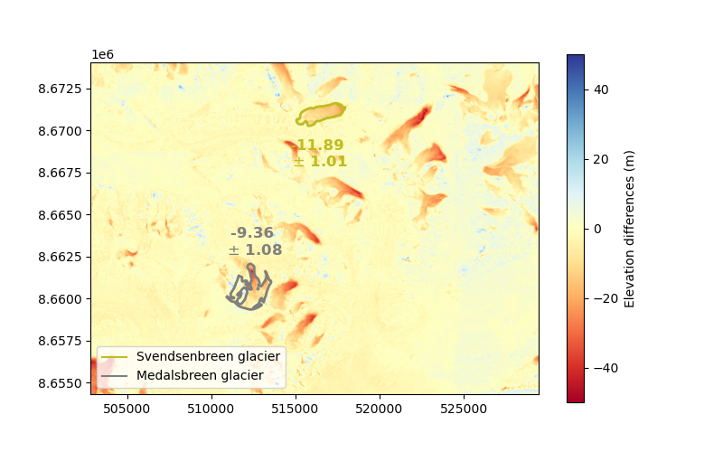
Because of slightly higher slopes and curvatures, the final uncertainty for Medalsbreen is larger by about 10%. The differences between the mean terrain slope and curvatures of stable terrain and those of glaciers is quite limited on Svalbard. In high moutain terrain, such as the Alps or Himalayas, the difference between stable terrain and glaciers, and among glaciers, would be much larger.