Estimation and modelling of spatial variograms

Digital elevation models have errors that are often correlated in space. While many DEM studies used solely short-range variogram to estimate the correlation of elevation measurement errors (e.g., Howat et al. (2008) , Wang and Kääb (2015)), recent studies show that variograms of multiple ranges provide larger, more reliable estimates of spatial correlation for DEMs.

Here, we show an example in which we estimate the spatial correlation for a DEM difference at Longyearbyen, and its impact on the standard error with averaging area. We first estimate an empirical variogram with xdem.spatialstats.sample_empirical_variogram() based on routines of scikit-gstat. We then fit the empirical variogram with a sum of variogram models using xdem.spatialstats.fit_sum_model_variogram(). Finally, we perform spatial propagation for a range of averaging area using xdem.spatialstats.number_effective_samples(), and empirically validate the improved robustness of our results using xdem.spatialstats.patches_method(), an intensive Monte-Carlo sampling approach.

Reference: Hugonnet et al. (2022), Figure 5 and Equations 13–16.

import geoutils as gu

import matplotlib.pyplot as plt
import numpy as np

import xdem
from xdem.spatialstats import nmad

We load example files.

dh = xdem.DEM(xdem.examples.get_path("longyearbyen_ddem"))
glacier_outlines = gu.Vector(xdem.examples.get_path("longyearbyen_glacier_outlines"))
mask_glacier = glacier_outlines.create_mask(dh)

We exclude values on glacier terrain in order to isolate stable terrain, our proxy for elevation errors.

dh.set_mask(mask_glacier)

We estimate the average per-pixel elevation error on stable terrain, using both the standard deviation and normalized median absolute deviation. For this example, we do not account for elevation heteroscedasticity.

print(f"STD: {np.nanstd(dh.data):.2f} meters.")
print(f"NMAD: {xdem.spatialstats.nmad(dh.data):.2f} meters.")

STD: 3.22 meters.
NMAD: 2.51 meters.

The two measures of dispersion are quite similar showing that, on average, there is a small influence of outliers on the elevation differences. The per-pixel precision is about \(\pm\) 2.5 meters. Does this mean that every pixel has an independent measurement error of \(\pm\) 2.5 meters? Let’s plot the elevation differences to visually check the quality of the data.

plt.figure(figsize=(8, 5))
dh.plot(ax=plt.gca(), cmap="RdYlBu", vmin=-4, vmax=4, cbar_title="Elevation differences (m)")

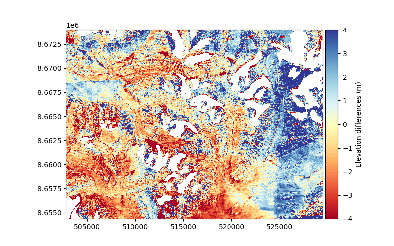
We clearly see that the residual elevation differences on stable terrain are not random. The positive and negative differences (blue and red, respectively) appear correlated over large distances. These correlated errors are what we want to estimate and model.

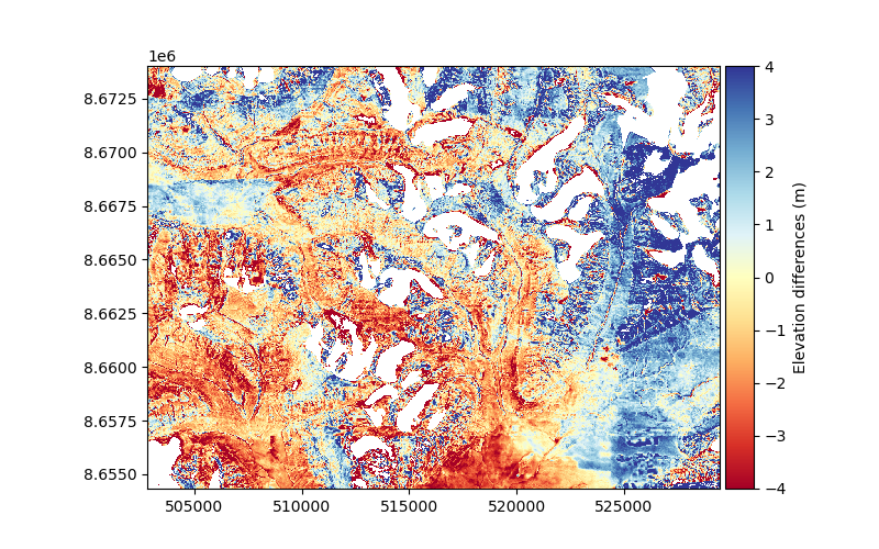
Additionally, we notice that the elevation differences are still polluted by unrealistically large elevation differences near glaciers, probably because the glacier inventory is more recent than the data, hence with too small outlines. To remedy this, we filter large elevation differences outside 4 NMAD.

dh.set_mask(np.abs(dh.data) > 4 * xdem.spatialstats.nmad(dh.data))

We plot the elevation differences after filtering to check that we successively removed glacier signals.

plt.figure(figsize=(8, 5))
dh.plot(ax=plt.gca(), cmap="RdYlBu", vmin=-4, vmax=4, cbar_title="Elevation differences (m)")

To quantify the spatial correlation of the data, we sample an empirical variogram. The empirical variogram describes the variance between the elevation differences of pairs of pixels depending on their distance. This distance between pairs of pixels if referred to as spatial lag.

To perform this procedure effectively, we use improved methods that provide efficient pairwise sampling methods for large grid data in scikit-gstat, which are encapsulated conveniently by xdem.spatialstats.sample_empirical_variogram(): Dowd’s variogram is used for robustness in conjunction with the NMAD (see Measures of spatial autocorrelation).

df = xdem.spatialstats.sample_empirical_variogram(
    values=dh, subsample=1000, n_variograms=10, estimator="dowd", random_state=42
)

Note: in this example, we add a random_state argument to yield a reproducible random sampling of pixels within the grid.

We plot the empirical variogram:

xdem.spatialstats.plot_variogram(df)

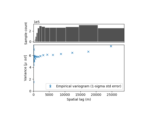
With this plot, it is hard to conclude anything! Properly visualizing the empirical variogram is one of the most important step. With grid data, we expect short-range correlations close to the resolution of the grid (~20-200 meters), but also possibly longer range correlation due to instrument noise or alignment issues (~1-50 km).

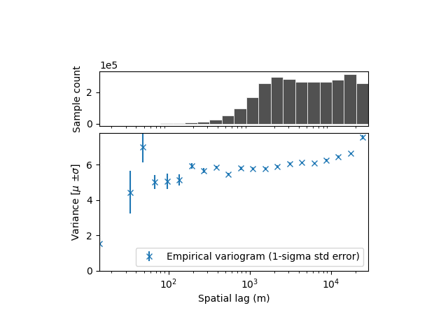
To better visualize the variogram, we can either change the axis to log-scale, but this might make it more difficult to later compare to variogram models. # Another solution is to split the variogram plot into subpanels, each with its own linear scale. Both are shown below.

Log scale:

xdem.spatialstats.plot_variogram(df, xscale="log")

Subpanels with linear scale:

xdem.spatialstats.plot_variogram(df, xscale_range_split=[100, 1000, 10000])

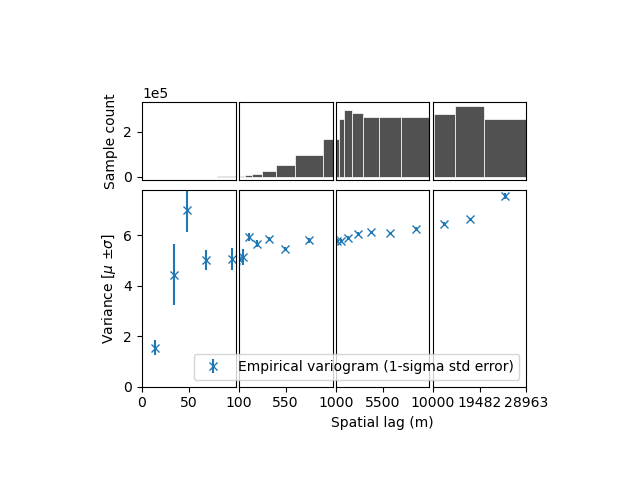
We identify:

• a short-range (i.e., correlation length) correlation, likely due to effects of resolution. It has a large partial sill (correlated variance), meaning that the elevation measurement errors are strongly correlated until a range of ~100 m.

• a longer range correlation, with a smaller partial sill, meaning the part of the elevation measurement errors remain correlated over a longer distance.

In order to show the difference between accounting only for the most noticeable, short-range correlation, or adding the long-range correlation, we fit this empirical variogram with two different models: a single spherical model, and the sum of two spherical models (two ranges). For this, we use xdem.spatialstats.fit_sum_model_variogram(), which is based on scipy.optimize.curve_fit:

func_sum_vgm1, params_vgm1 = xdem.spatialstats.fit_sum_model_variogram(
    list_models=["Spherical"], empirical_variogram=df
)

func_sum_vgm2, params_vgm2 = xdem.spatialstats.fit_sum_model_variogram(
    list_models=["Spherical", "Spherical"], empirical_variogram=df
)

xdem.spatialstats.plot_variogram(
    df,
    list_fit_fun=[func_sum_vgm1, func_sum_vgm2],
    list_fit_fun_label=["Single-range model", "Double-range model"],
    xscale_range_split=[100, 1000, 10000],
)

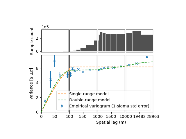
The sum of two spherical models fits better, accouting for the small partial sill at longer ranges. Yet this longer range partial sill (correlated variance) is quite small…

So one could wonder: is it really important to account for this small additional “bump” in the variogram?

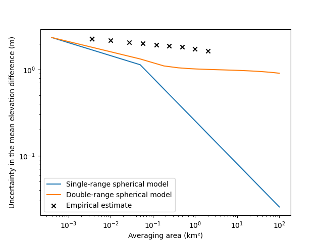
To answer this, we compute the precision of the DEM integrated over a certain surface area based on spatial integration of the variogram models using xdem.spatialstats.neff_circ(), with areas varying from pixel size to grid size. Numerical and exact integration of variogram is fast, allowing us to estimate errors for a wide range of areas rapidly.

areas = np.linspace(20, 10000, 50) ** 2

list_stderr_singlerange, list_stderr_doublerange, list_stderr_empirical = ([] for i in range(3))
for area in areas:

    # Number of effective samples integrated over the area for a single-range model
    neff_singlerange = xdem.spatialstats.number_effective_samples(area, params_vgm1)

    # For a double-range model
    neff_doublerange = xdem.spatialstats.number_effective_samples(area, params_vgm2)

    # Convert into a standard error
    stderr_singlerange = nmad(dh.data) / np.sqrt(neff_singlerange)
    stderr_doublerange = nmad(dh.data) / np.sqrt(neff_doublerange)
    list_stderr_singlerange.append(stderr_singlerange)
    list_stderr_doublerange.append(stderr_doublerange)

We add an empirical error based on intensive Monte-Carlo sampling (“patches” method) to validate our results. This method is implemented in xdem.spatialstats.patches_method(). Here, we sample fewer areas to avoid for the patches method to run over long processing times, increasing from areas of 5 pixels to areas of 10000 pixels exponentially.

areas_emp = [4000 * 2 ** (i) for i in range(10)]
df_patches = xdem.spatialstats.patches_method(dh, gsd=dh.res[0], areas=areas_emp)


fig, ax = plt.subplots()
plt.plot(np.asarray(areas) / 1000000, list_stderr_singlerange, label="Single-range spherical model")
plt.plot(np.asarray(areas) / 1000000, list_stderr_doublerange, label="Double-range spherical model")
plt.scatter(
    df_patches.exact_areas.values / 1000000,
    df_patches.nmad.values,
    label="Empirical estimate",
    color="black",
    marker="x",
)
plt.xlabel("Averaging area (km²)")
plt.ylabel("Uncertainty in the mean elevation difference (m)")
plt.xscale("log")
plt.yscale("log")
plt.legend()
plt.show()

Note: in this example, we add a random_state argument to the patches method to yield a reproducible random sampling, and set n_patches to reduce computing time.

Using a single-range variogram highly underestimates the measurement error integrated over an area, by over a factor of ~100 for large surface areas. Using a double-range variogram brings us closer to the empirical error.

But, in this case, the error is still too small. Why? The small size of the sampling area against the very large range of the noise implies that we might not verify the assumption of second-order stationarity (see spatialstats). Longer range correlations might be omitted by our analysis, due to the limits of the variogram sampling. In other words, a small part of the variance could be fully correlated over a large part of the grid: a vertical bias.

As a first guess for this, let’s examine the difference between mean and median to gain some insight on the central tendency of our sample:

diff_med_mean = np.nanmean(dh.data.data) - np.nanmedian(dh.data.data)
print(f"Difference mean/median: {diff_med_mean:.3f} meters.")

Difference mean/median: -0.821 meters.

If we now express it as a percentage of the dispersion:

print(f"{diff_med_mean/np.nanstd(dh.data)*100:.1f} % of STD.")

-30.3 % of STD.

There might be a significant bias of central tendency, i.e. almost fully correlated measurement error across the grid. If we assume that around 5% of the variance is fully correlated, and re-calculate our elevation measurement errors accordingly.

list_stderr_doublerange_plus_fullycorrelated = []
for area in areas:

    # For a double-range model
    neff_doublerange = xdem.spatialstats.neff_circular_approx_numerical(area=area, params_variogram_model=params_vgm2)

    # About 5% of the variance might be fully correlated, the other 95% has the random part that we quantified
    stderr_fullycorr = np.sqrt(0.05 * np.nanvar(dh.data))
    stderr_doublerange = np.sqrt(0.95 * np.nanvar(dh.data)) / np.sqrt(neff_doublerange)
    list_stderr_doublerange_plus_fullycorrelated.append(stderr_fullycorr + stderr_doublerange)

fig, ax = plt.subplots()
plt.plot(np.asarray(areas) / 1000000, list_stderr_singlerange, label="Single-range spherical model")
plt.plot(np.asarray(areas) / 1000000, list_stderr_doublerange, label="Double-range spherical model")
plt.plot(
    np.asarray(areas) / 1000000,
    list_stderr_doublerange_plus_fullycorrelated,
    label="5% fully correlated,\n 95% double-range spherical model",
)
plt.scatter(
    df_patches.exact_areas.values / 1000000,
    df_patches.nmad.values,
    label="Empirical estimate",
    color="black",
    marker="x",
)
plt.xlabel("Averaging area (km²)")
plt.ylabel("Uncertainty in the mean elevation difference (m)")
plt.xscale("log")
plt.yscale("log")
plt.legend()
plt.show()

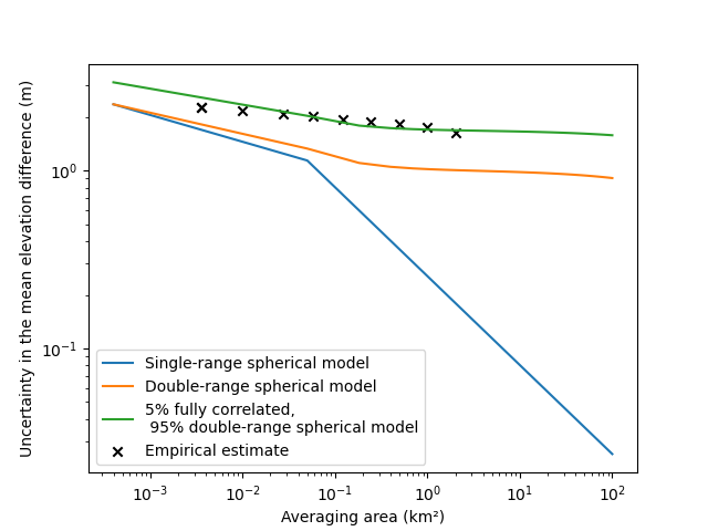
Our final estimation is now very close to the empirical error estimate.

Some take-home points:

1. Long-range correlations are very important to reliably estimate measurement errors integrated in space, even if they have a small partial sill i.e. correlated variance,

2. Ideally, the grid must only contain correlation patterns significantly smaller than the grid size to verify second-order stationarity. Otherwise, be wary of small biases of central tendency, i.e. fully correlated measurement errors!