Uncertainty analysis#
xDEM integrates uncertainty analysis tools from the recent literature that rely on joint methods from two scientific fields: spatial statistics and uncertainty quantification.
While uncertainty analysis technically refers to both systematic and random errors, systematic errors of elevation data are corrected using Coregistration and Bias correction, so we here refer to uncertainty analysis for quantifying and propagating random errors (including structured errors).
In detail, xDEM provides tools to:
Estimate and model elevation heteroscedasticity, i.e. variable random errors (e.g., such as with terrain slope or stereo-correlation),
Estimate and model the spatial correlation of random errors (e.g., from native spatial resolution or instrument noise),
Perform error propagation to elevation derivatives (e.g., spatial average, or more complex derivatives such as slope and aspect).
More reading
For an introduction on spatial statistics applied to uncertainty quantification for elevation data, we recommend reading the Spatial statistics for error analysis guide page and, for details on variography, the documentation of SciKit-GStat.
Additionally, we recommend reading the Static surfaces as error proxy guide page on which uncertainty analysis relies.
Quick use#
The estimation of the spatial structure of random errors of elevation data is conveniently
wrapped in a single method estimate_uncertainty(), which estimates, models and returns a map of
variable error matching the DEM, and a function describing the spatial correlation of these errors.
# Estimate elevation uncertainty assuming both DEMs have similar precision
sig_dem, rho_sig = tba_dem_coreg.estimate_uncertainty(ref_dem, stable_terrain=inlier_mask, precision_of_other="same", random_state=42)

# The error map variability is estimated from slope and curvature by default
sig_dem.plot(cmap="Purples", cbar_title=r"Error in elevation (1$\sigma$, m)")

# The spatial correlation function represents how much errors are correlated at a certain distance
print("Random elevation errors at a distance of 1 km are correlated at {:.2f} %.".format(rho_sig(1000) * 100))
Random elevation errors at a distance of 1 km are correlated at 14.81 %.

Three methods can be considered for this estimation, which are described right below. Additionally, the subfunctions used to perform the uncertainty analysis are detailed in the Spatial structure of error section below.
Summary of available methods#
Methods for modelling the structure of error are based on spatial statistics, and methods for propagating errors to spatial derivatives analytically rely on uncertainty propagation.
To improve the robustness of the uncertainty analysis, we provide refined frameworks for application to elevation data based on Rolstad et al. (2009) and Hugonnet et al. (2022), both for modelling the structure of error and to efficiently perform error propagation. These frameworks are generic, simply extending an aspect of the uncertainty analysis to better work on elevation data, and thus generally encompass methods described in other studies on the topic (e.g., Anderson et al. (2019)).
The tables below summarize the characteristics of these methods.
Estimating and modeling the structure of error#
Frequently, in spatial statistics, a single correlation range is considered (“basic” method below). However, elevation data often contains errors with correlation ranges spanning different orders of magnitude. For this, Rolstad et al. (2009) and Hugonnet et al. (2022) consider potential multiple ranges of spatial correlation (instead of a single one). In addition, Hugonnet et al. (2022) considers potential heteroscedasticity or variable errors (instead of homoscedasticity, or constant errors), also common in elevation data.
Because accounting for possible multiple correlation ranges also works if you have a single correlation range in your data, and accounting for potential heteroscedasticity also works on homoscedastic data, there is little to lose by using a more advanced framework! (most often, only a bit of additional computation time)
Method |
Heteroscedasticity (i.e. variable error) |
Correlations (single-range) |
Correlations (multi-range) |
|---|---|---|---|
Basic |
❌ |
✅ |
❌ |
R2009 |
❌ |
✅ |
✅ |
H2022 (default) |
✅ |
✅ |
✅ |
For consistency, all methods default to robust estimators: the normalized median absolute deviation (NMAD) for the spread, and Dowd’s estimator for the variogram. See the Need for robust estimators guide page for details.
Propagating errors to spatial derivatives#
Exact uncertainty propagation scales exponentially with data (by computing every pairwise combinations, for potentially millions of elevation data points or pixels). To remedy this, Rolstad et al. (2009) and Hugonnet et al. (2022) both provide an approximation of exact uncertainty propagations for spatial derivatives (to avoid long computing times). These approximations are valid in different contexts, described below.
Method |
Accuracy |
Computing time |
Validity |
|---|---|---|---|
Exact discretized |
Exact |
Slow on large samples (exponential complexity) |
Always |
R2009 |
Conservative |
Instantaneous (numerical integration) |
Only for near-circular contiguous areas |
H2022 (default) |
Accurate |
Fast (linear complexity) |
As long as variance is nearly stationary |
Core concept for error proxy#
Below, we examplify the different steps of uncertainty analysis of elevation differences between two datasets on static surfaces as an error proxy.
In case you want to convert the uncertainties of elevation differences into that of a “target” elevation dataset, it can be either assumed that:
The “other” elevation dataset is much more precise, in which case the uncertainties in elevation differences directly approximate that of the “target” elevation dataset,
The “other” elevation dataset has similar precision, in which case the uncertainties of elevation differences quadratically combine twice that of the “target” elevation dataset.
More reading (reminder)
To clarify these conversions of error proxy, see the Static surfaces as error proxy guide page. For more statistical background on the methods below, see the Spatial statistics for error analysis guide page.
Spatial structure of error#
Below we detail the steps used to estimate the two components of uncertainty: heteroscedasticity and spatial
correlation of errors in estimate_uncertainty(), as these are most easily customized
by calling their subfunctions independently.
Important
Some uncertainty functionalities are being adapted to operate directly in SciKit-GStat (e.g., fitting a sum of
variogram models, pairwise subsampling for grid data). This will allow to simplify function inputs and outputs of xDEM,
for instance by relying on a single, consistent Variogram() object.
This will trigger API changes in future package versions.
Heteroscedasticity#
The first component of uncertainty is the estimation and modelling of elevation
heteroscedasticity (or variability in
random elevation errors) through infer_heteroscedasticity_from_stable(), which has three steps.
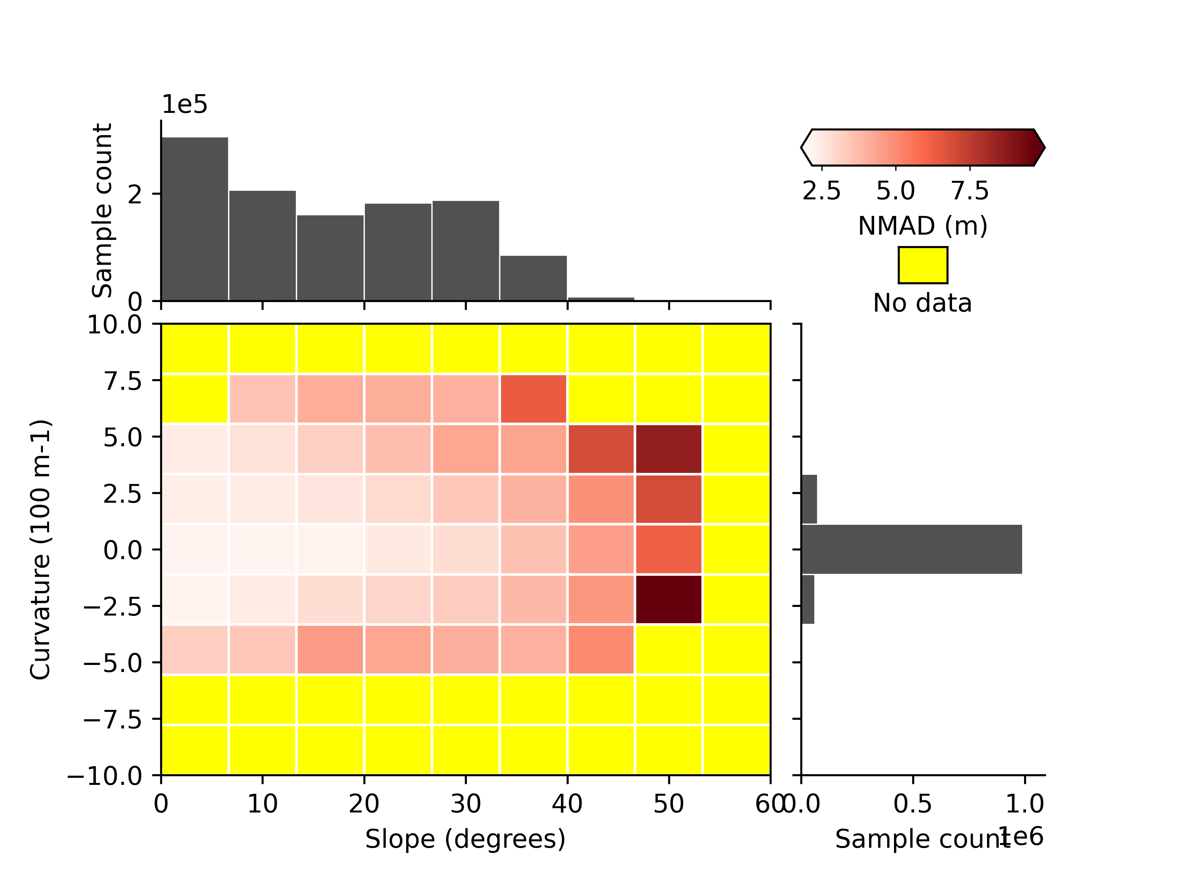
Step 1: Empirical estimation of heteroscedasticity
The variability in errors is empirically estimated by data binning
in N-dimensions of the elevation differences on stable terrain, using the function nd_binning().
Plotting of 1- and 2D binnings can be facilitated by the functions plot_1d_binning() and
plot_2d_binning().
The most common explanatory variables for elevation heteroscedasticity are the terrain slope and curvature (used as default, see Terrain attributes), and other quality metrics passed by the user such as the correlation (for stereo DEMs) or the interferometric coherence (for InSAR DEMs).
# Get elevation differences and stable terrain mask
dh = ref_dem - tba_dem_coreg
glacier_outlines = gu.Vector(xdem.examples.get_path("longyearbyen_glacier_outlines"))
stable_terrain = ~glacier_outlines.create_mask(dh)

# Derive slope and curvature
slope, curv = ref_dem.get_terrain_attribute(attribute=["slope", "curvature"])

# Use only array of stable terrain
dh_arr = dh[stable_terrain]
slope_arr = slope[stable_terrain]
curv_arr = curv[stable_terrain]

# Estimate the variable error by bin of slope and curvature
df_h = xdem.spatialstats.nd_binning(
    dh_arr, list_var=[slope_arr, curv_arr], list_var_names=["slope", "curv"], statistics=["count", gu.stats.nmad], list_var_bins=[np.linspace(0, 60, 10), np.linspace(-10, 10, 10)]
)

# Plot 2D binning
xdem.spatialstats.plot_2d_binning(df_h, "slope", "curv", "nmad", "Slope (degrees)", "Curvature (100 m-1)", "NMAD (m)")
Step 2: Modelling of the heteroscedasticity
Once empirically estimated, elevation heteroscedasticity can be modelled either by a function fit, or by
N-D linear interpolation using interp_nd_binning(), in order to yield a value for any slope
and curvature:
# Derive a numerical function of the measurement error
sig_dh_func = xdem.spatialstats.interp_nd_binning(df_h, list_var_names=["slope", "curv"])
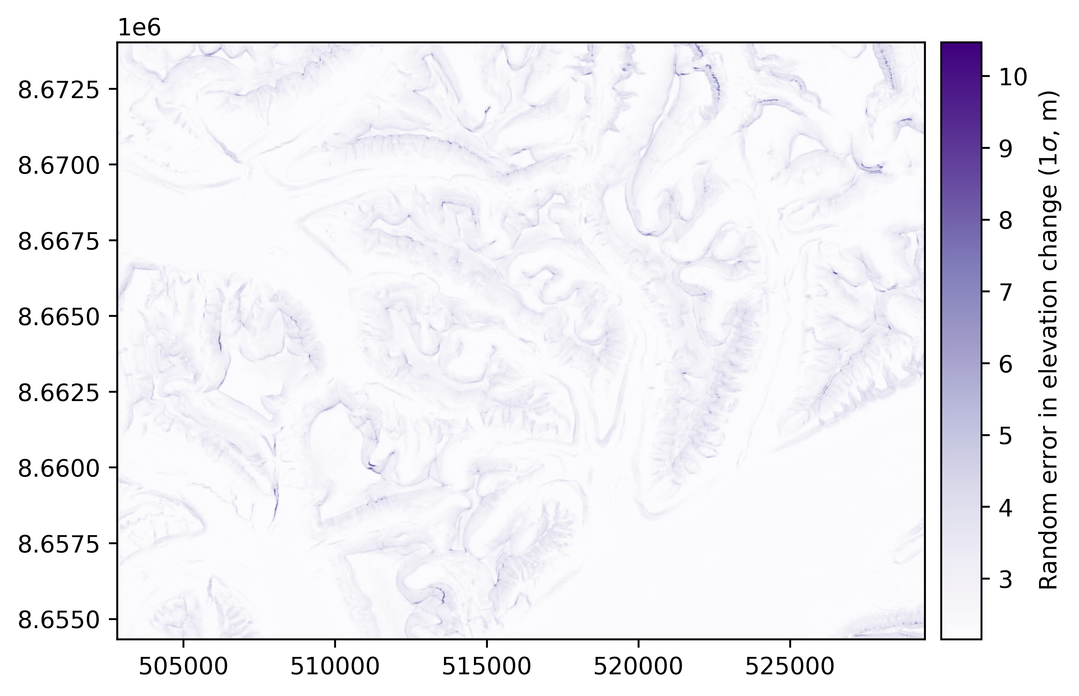
Step 3: Applying the model
Using the model, we can estimate the random error on all terrain using their slope and curvature, and derive a map of random errors in elevation change:
# Apply function to the slope and curvature on all terrain
sig_dh_arr = sig_dh_func((slope.data, curv.data))

# Convert to raster and plot
sig_dh = dh.copy(new_array=sig_dh_arr)
sig_dh.plot(cmap="Purples", cbar_title=r"Random error in elevation change (1$\sigma$, m)")
Spatial correlation of errors#
The second component of uncertainty is the estimation and modelling of spatial correlations of random errors through
infer_spatial_correlation_from_stable(), which has three steps.
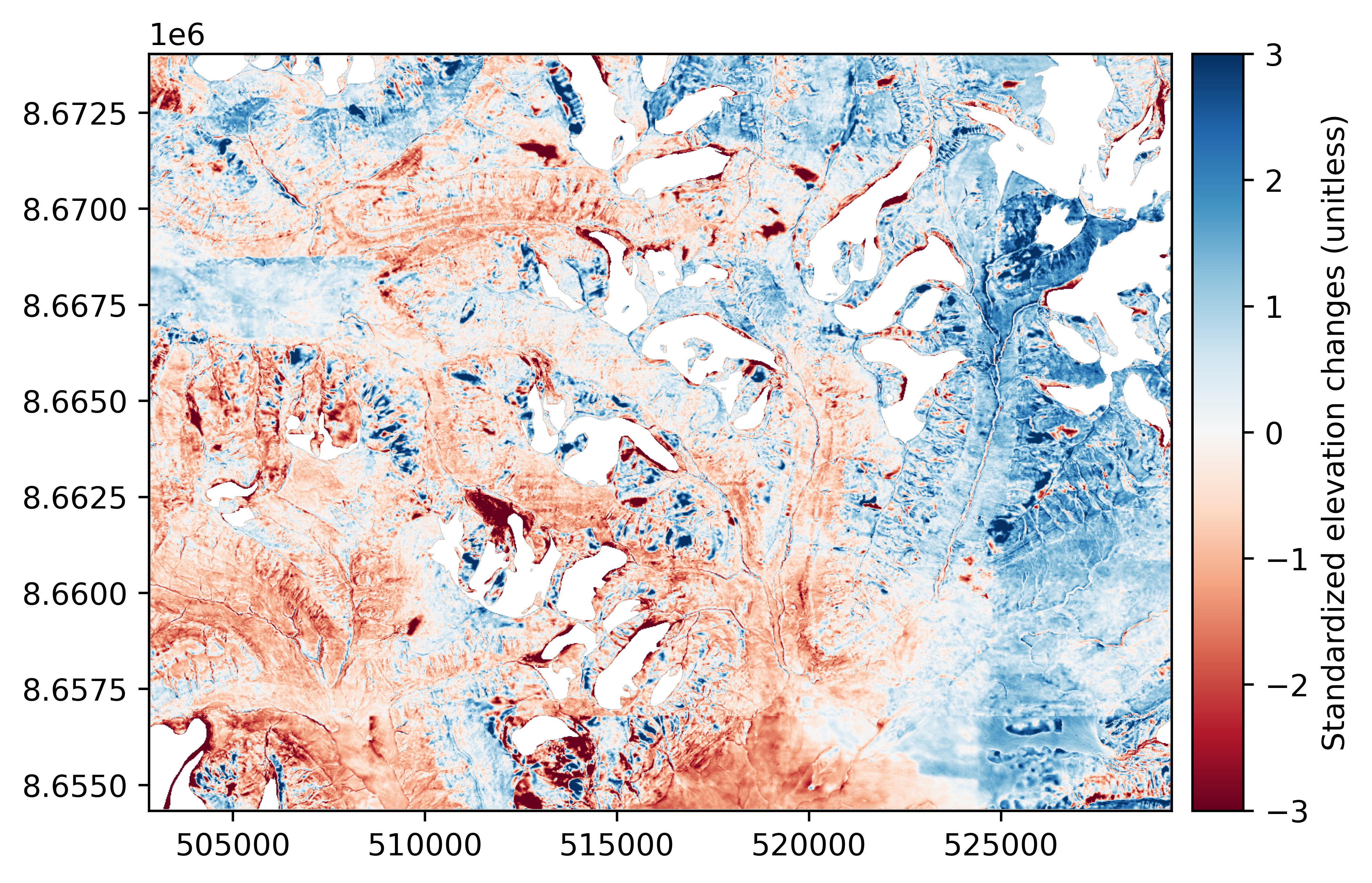
Step 1: Standardization
If heteroscedasticity was considered, elevation differences can be standardized by the variable error to reduce its influence on the estimation of spatial correlations. Otherwise, elevation differences are used directly.
# Standardize the data
z_dh = dh / sig_dh
# Mask values to keep only stable terrain
z_dh.set_mask(~stable_terrain)
# Plot the standardized data on stable terrain
z_dh.plot(cmap="RdBu", vmin=-3, vmax=3, cbar_title="Standardized elevation changes (unitless)")
Step 2: Empirical estimation of the variogram
An empirical variogram can be estimated with sample_empirical_variogram().
# Sample empirical variogram
df_vgm = xdem.spatialstats.sample_empirical_variogram(values=z_dh, subsample=500, n_variograms=5, random_state=42)
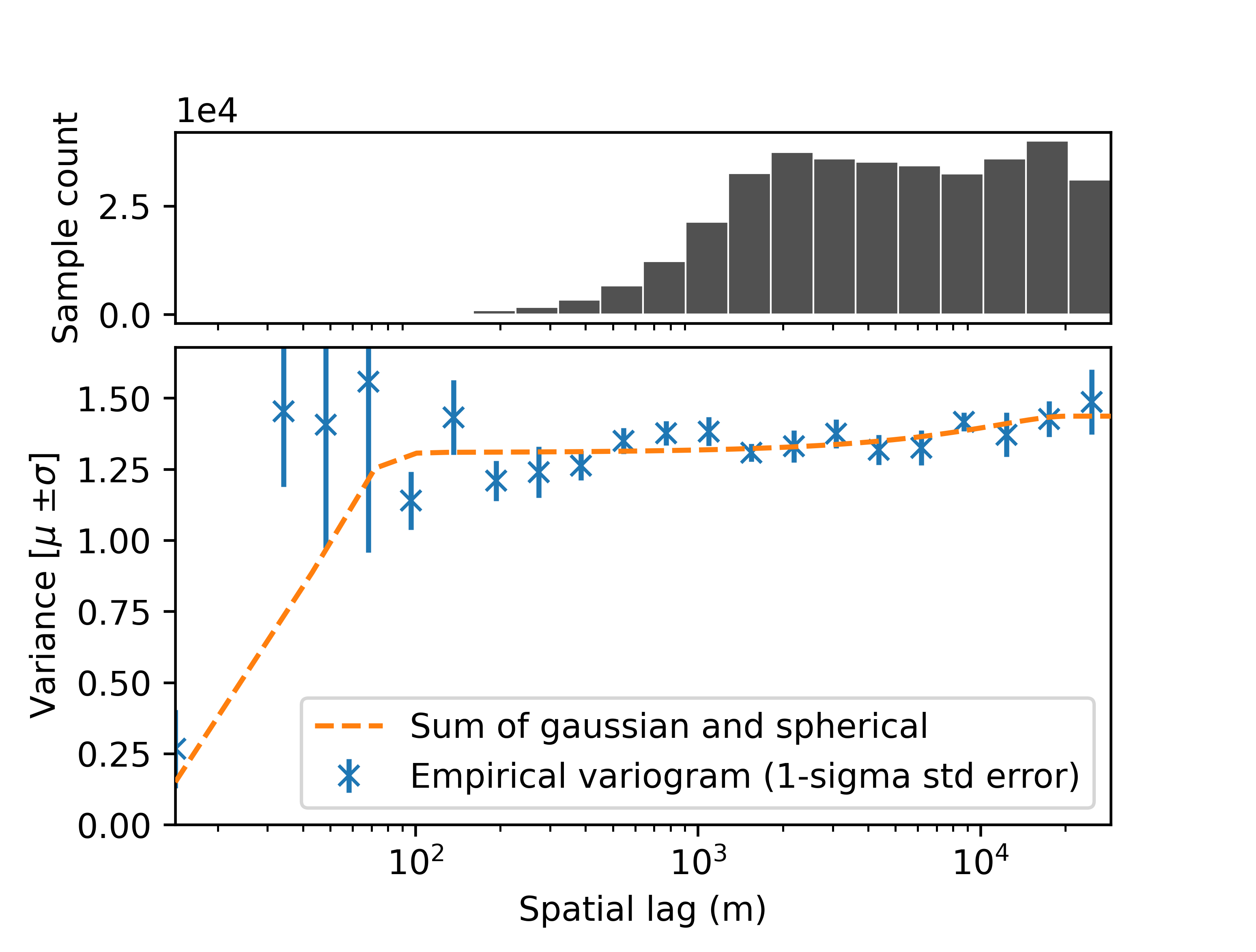
Step 3: Modelling of the variogram
Once empirically estimated, the variogram can be modelled by a functional form with fit_sum_model_variogram().
Plotting of the empirical and modelled variograms is facilitated by plot_variogram().
# Fit the sum of a gaussian and spherical model
func_sum_vgm, params_variogram_model = xdem.spatialstats.fit_sum_model_variogram(
    list_models=["Gaussian", "Spherical"], empirical_variogram=df_vgm
)
# Plot empirical and modelled variogram
xdem.spatialstats.plot_variogram(df_vgm, [func_sum_vgm], ["Sum of gaussian and spherical"], xscale="log")
Propagation of errors#
The two uncertainty components estimated above allow to propagate elevation errors. xDEM provides methods to theoretically propagate errors to spatial derivatives (mean or sum in an area), with efficient computing times. For more complex derivatives (such as terrain attributes), we recommend to combine the structure of error defined above with random field simulation methods available in packages such as GSTools.
Spatial derivatives#
The propagation of random errors to a spatial derivative is done with
spatial_error_propagation(), which divides into three steps.
Each step derives a part of the standard error in the area. For example, for the error of the mean elevation difference \(\sigma_{\overline{dh}}\):
# Get an area of interest where we want to propagate errors
outline_brom = gu.Vector(glacier_outlines.ds[glacier_outlines.ds["NAME"] == "Brombreen"])
mask_brom = outline_brom.create_mask(dh)
Step 1: Account for variable error
We compute the mean of the variable random error in the area \(\overline{\sigma_{dh}}\).
# Calculate the mean random error in the area
mean_sig = np.nanmean(sig_dh[mask_brom])
Step 2: Account for spatial correlation
We estimate the number of effective samples in the area \(N_{eff}\) due to the spatial correlations.
Note
We notice a warning below: The resolution for rasterizing the outline was automatically chosen based on the short correlation range.
# Calculate the area-averaged uncertainty with these models
neff = xdem.spatialstats.number_effective_samples(area=outline_brom, params_variogram_model=params_variogram_model)
UserWarning: Resolution for vector rasterization is not defined and thus set at 20% of the shortest correlation range, which might result in large memory usage.
Step 3: Derive final error
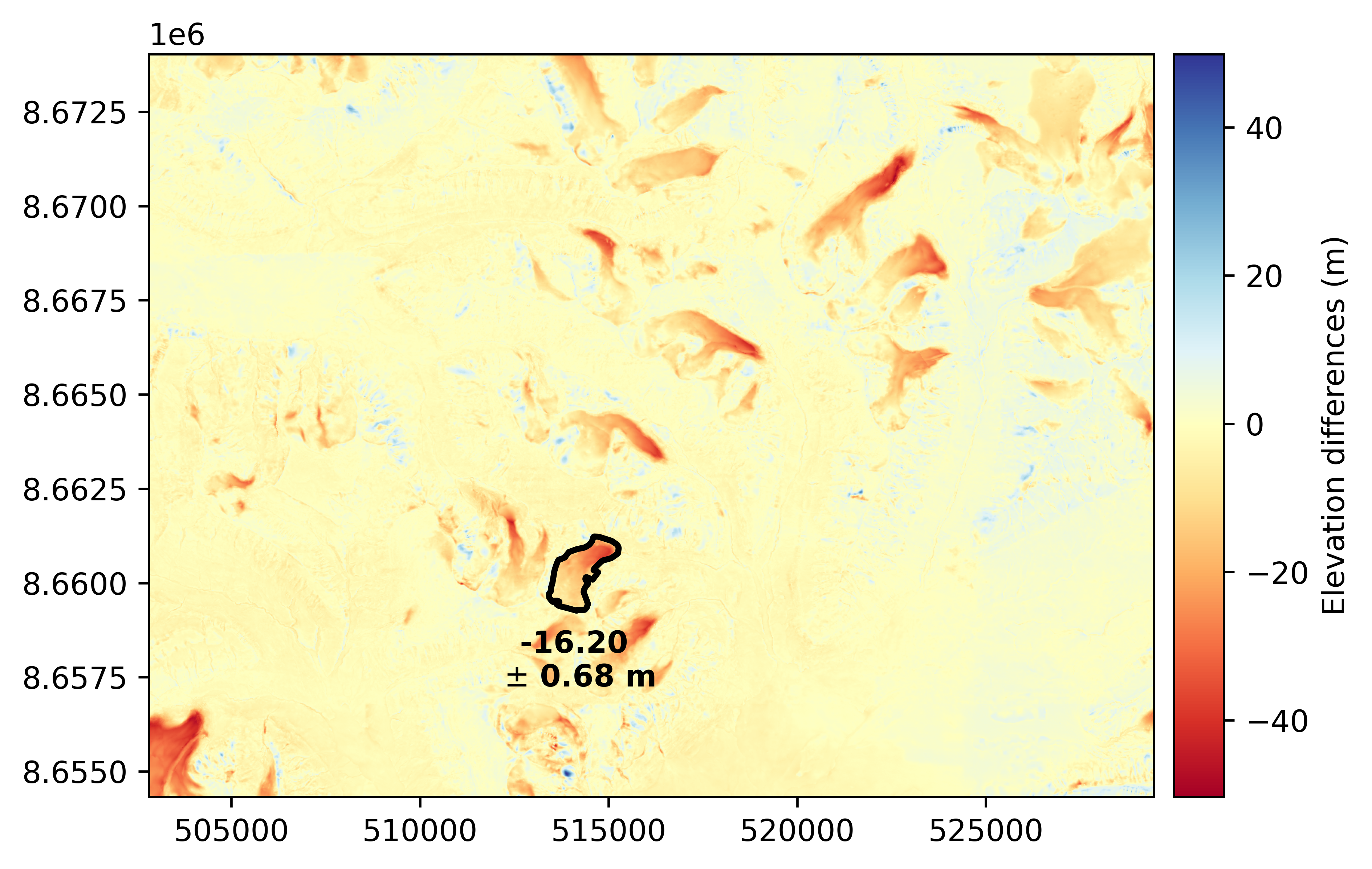
And we can now compute our final random error for the mean elevation change in this area of interest:
# Compute the standard error
sig_dh_brom = mean_sig / np.sqrt(neff)

# Mean elevation difference
dh_brom = np.nanmean(dh[mask_brom])

# Plot the result
dh.plot(cmap="RdYlBu", cbar_title="Elevation differences (m)")
outline_brom.plot(dh, fc="none", ec="black", lw=2)
plt.text(
    outline_brom.ds.centroid.x.values[0],
    outline_brom.ds.centroid.y.values[0] - 1500,
    f"{dh_brom:.2f} \n$\\pm$ {sig_dh_brom:.2f} m",
    color="black",
    fontweight="bold",
    va="top",
    ha="center",
)
plt.show()