Cheatsheet: How to correct… ?#
In elevation data analysis, the problem generally starts with identifying what correction method to apply when observing a specific pattern of error in your own data.
Below, we summarize a cheatsheet that links what method is likely to correct a pattern of error you can visually identify on a map of elevation differences with another elevation dataset (looking at static surfaces)!
Cheatsheet#
The patterns of error categories listed in this spreadsheet are linked to visual examples further below that you can use to compare to your own elevation differences.
Pattern |
Description |
Cause and correction |
Notes |
|---|---|---|---|
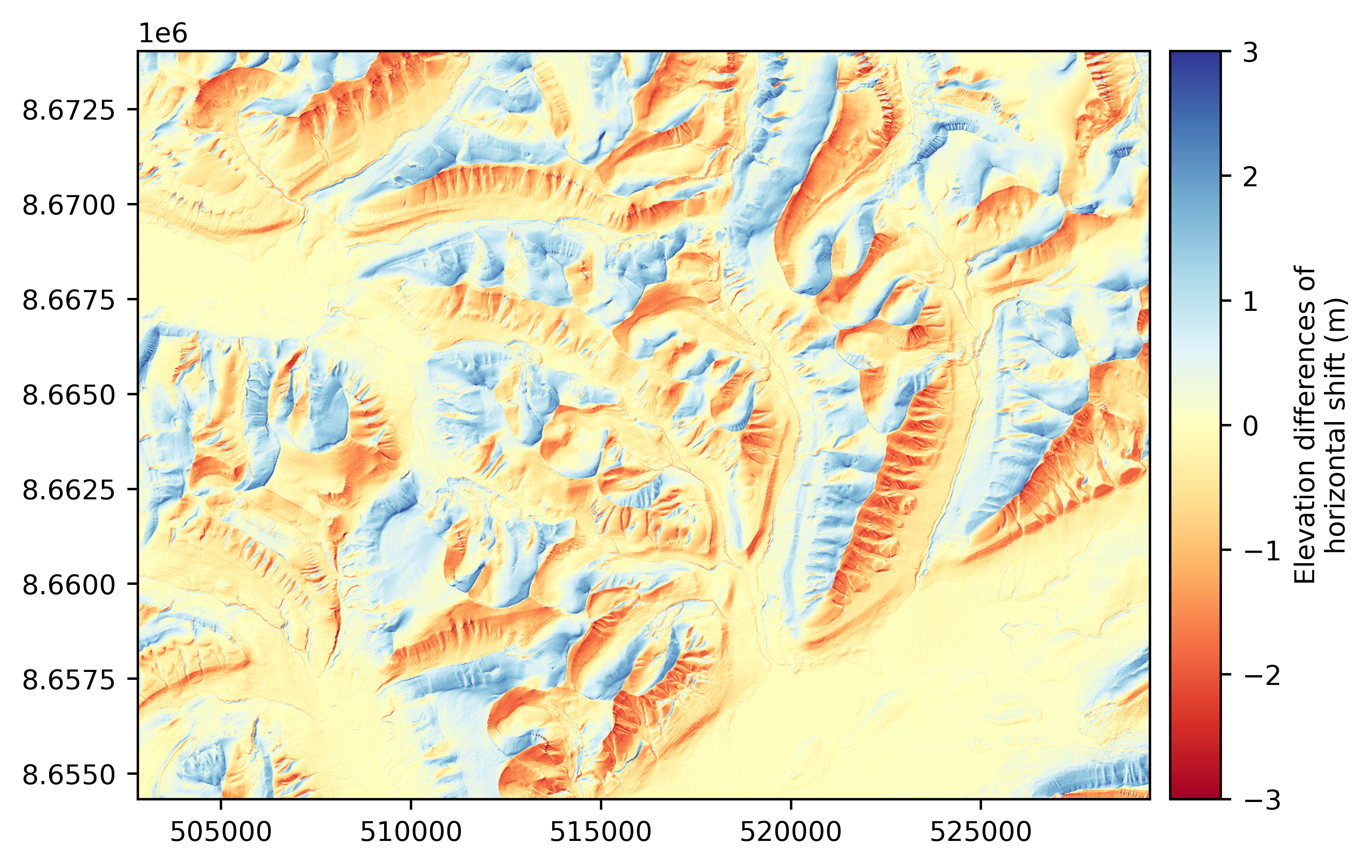
Positive and negative errors that are larger near high slopes and symmetric with opposite slope orientation, making landforms appear visually. |
Likely horizontal shift due to geopositioning errors, use a Coregistration such as |
Even a tiny horizontal misalignment can be visually identified! To not confuse with Peak cuts and cavity fills. |
|
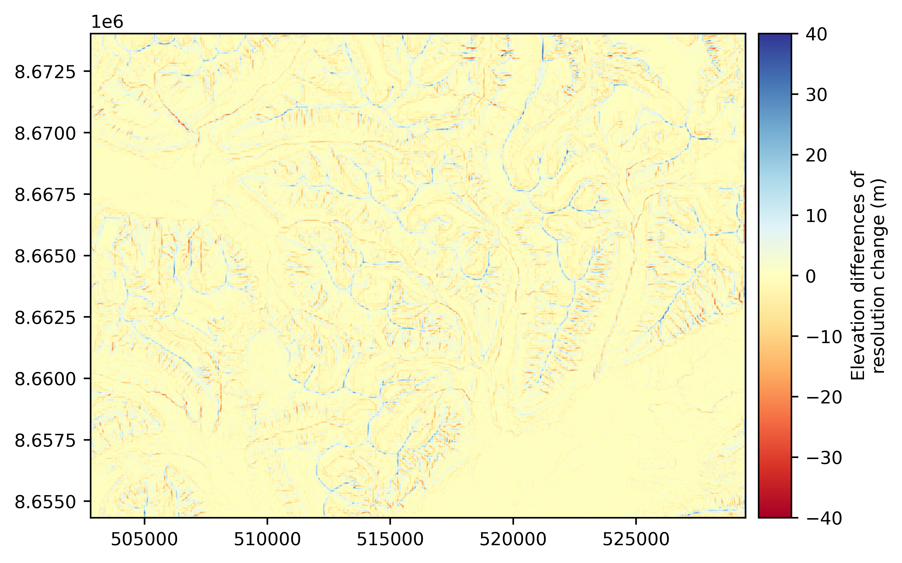
Positive and negative errors, with one sign located exclusively near peaks and the other exclusively near cavities. |
Likely resolution-type errors, use a Bias correction such as |
Can be over-corrected, sometimes better to simply ignore during analysis. Or avoid by downsampling all elevation data to the lowest resolution, rather than upsampling to the highest. |
|
Smooth offsets varying at scale of 10 km+, often same sign (either positive or negative). |
Likely wrong Vertical referencing, can set and transform with |
Vertical references often only exists in a user guide, they are not coded in the raster CRS and need to be set manually. |
|
Ramping errors, often near the edge of the data extent, sometimes with a center dome. |
Likely ramp/rotations due to camera errors, use either a Coregistration such as |
Can sometimes be more rigorously fixed ahead of DEM generation with bundle adjustment. |
|
Positive and negative errors undulating patterns at one or several frequencies well larger than pixel size. |
Likely jitter-type errors, use a Bias correction such as |
Can sometimes be more rigorously fixed ahead of DEM generation with jitter correction. |
|
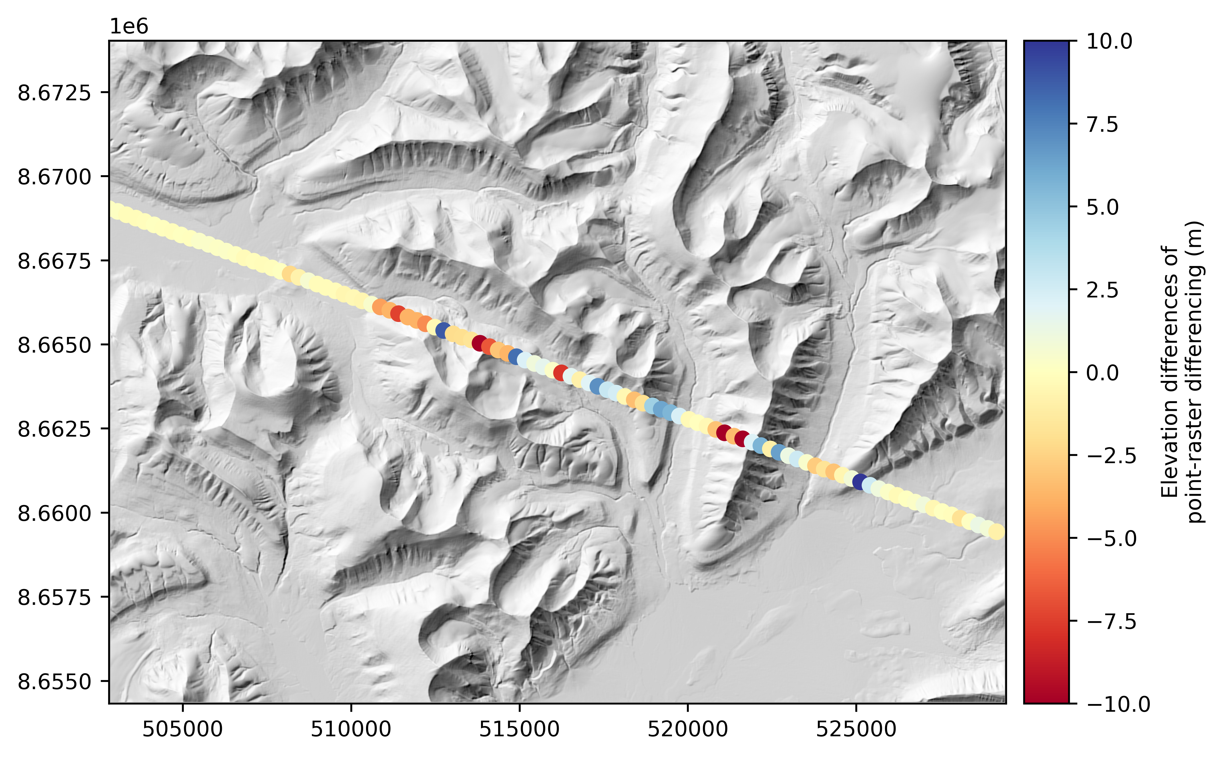
Point data errors that alternate between negative and positive, higher on steeper slopes. |
Likely wrong point-raster comparison, use point interpolation or reduction on the raster instead such as |
Rasterizing point data introduces spatially correlated random errors, instead it is recommended to interpolate raster data at the point coordinates. |
Visual patterns of errors#
Important
The patterns of errors below are created synthetically to examplify the effect of a single source of error. In your own elevation differences, those will be mixed together and with random errors inherent to the data.
For examples on real data, see the Basic and Advanced gallery examples!
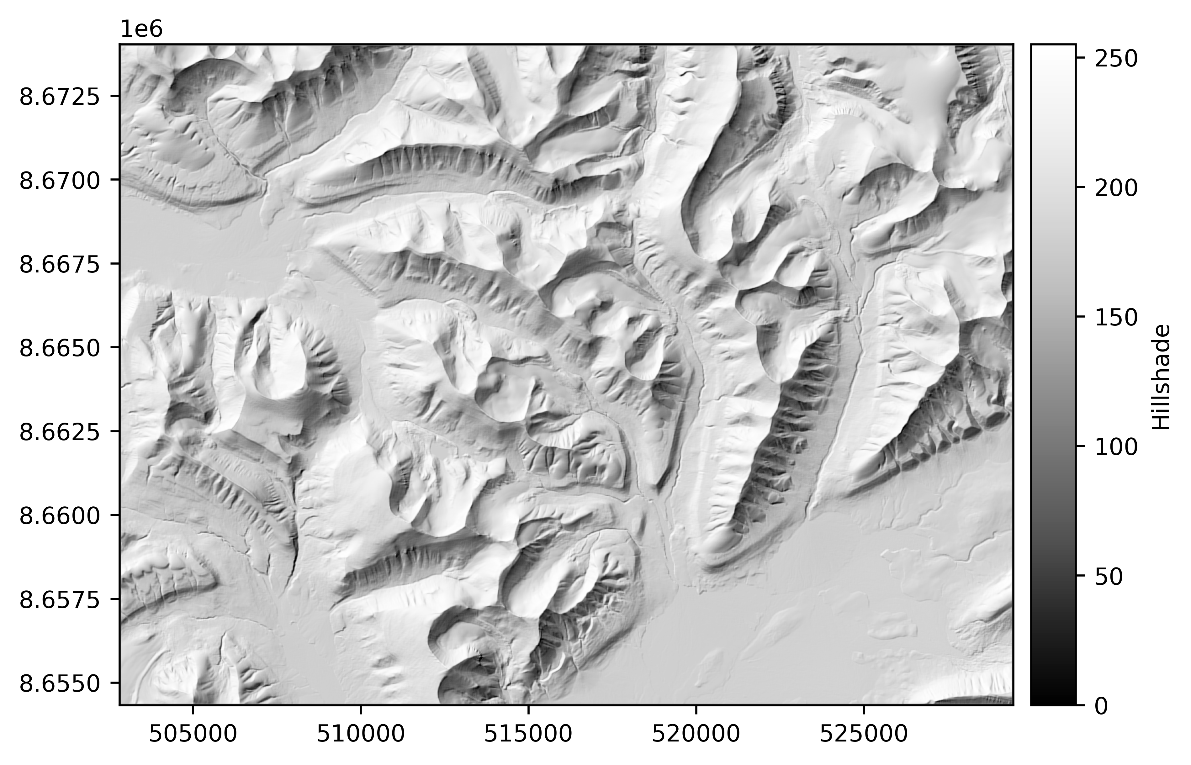
It is often crucial to relate the location of your errors on static surfaces to the terrain distribution (in particular, its slope and curvature), which can usually be inferred visually from a hillshade.
hs = dem.hillshade()
hs.plot(cmap="Greys_r", cbar_title="Hillshade")
Sharp landforms#
Example of sharp landforms appearing with a horizontal shift due to geolocation errors. We here translate the DEM horizontally by 1/10th of a pixel, for a pixel resolution of 20 m.
Peak cuts and cavity fills#
Example of peak cutting and cavity filling errors. We here downsampled our DEM from 20 m to 100 m to simulate a lower native resolution, then upsample it again to 20 m, to show the errors affect areas near high curvatures such as peaks and cavities.
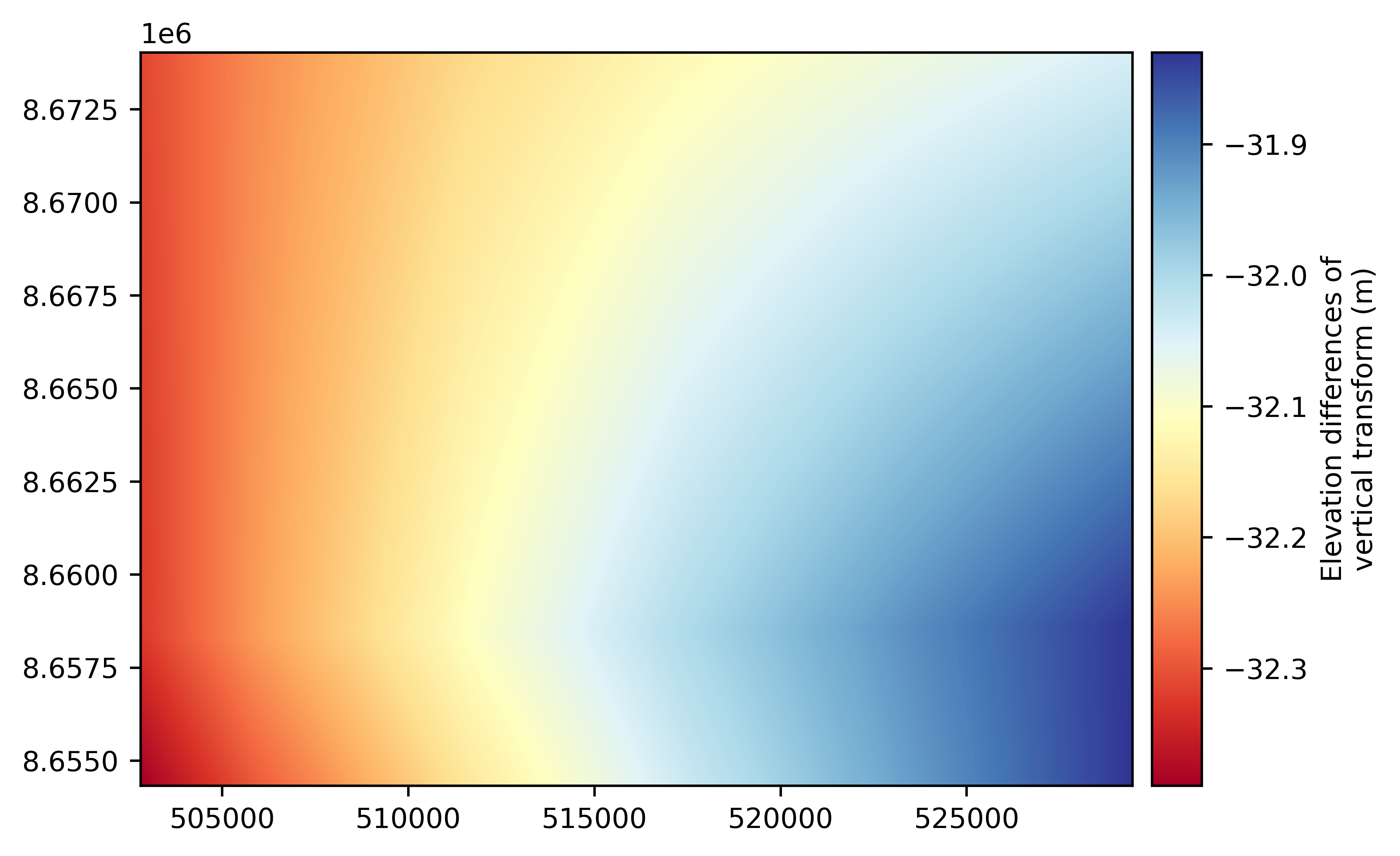
Smooth-field offset#
Example of smooth large offset field created by a wrong vertical CRS. We here show the difference due to the EGM96 geoid added on top of the ellipsoid.
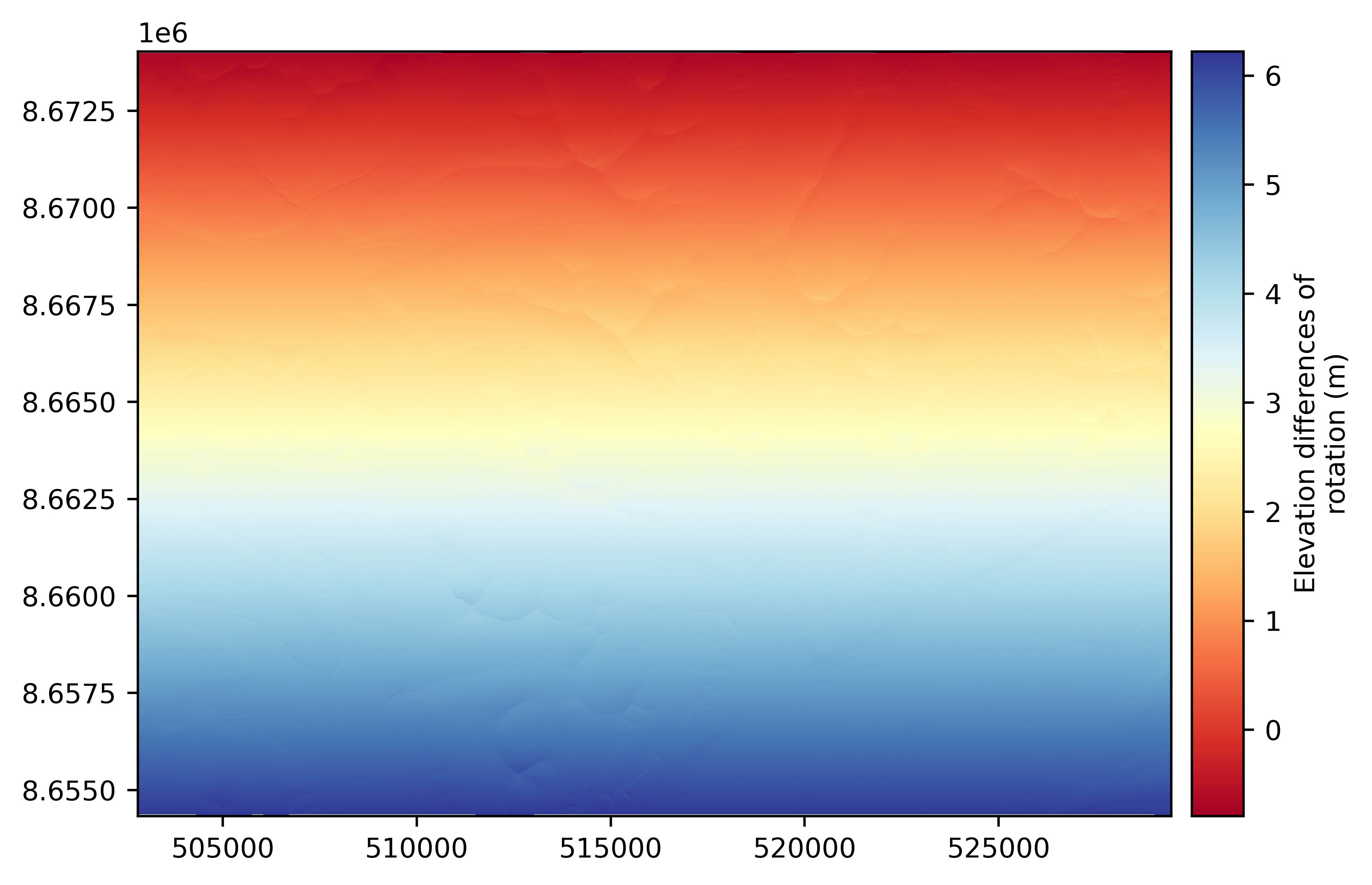
Ramp or dome#
Example of ramp created by a rotation due to camera errors. We here show just a slight rotation of 0.02 degrees.
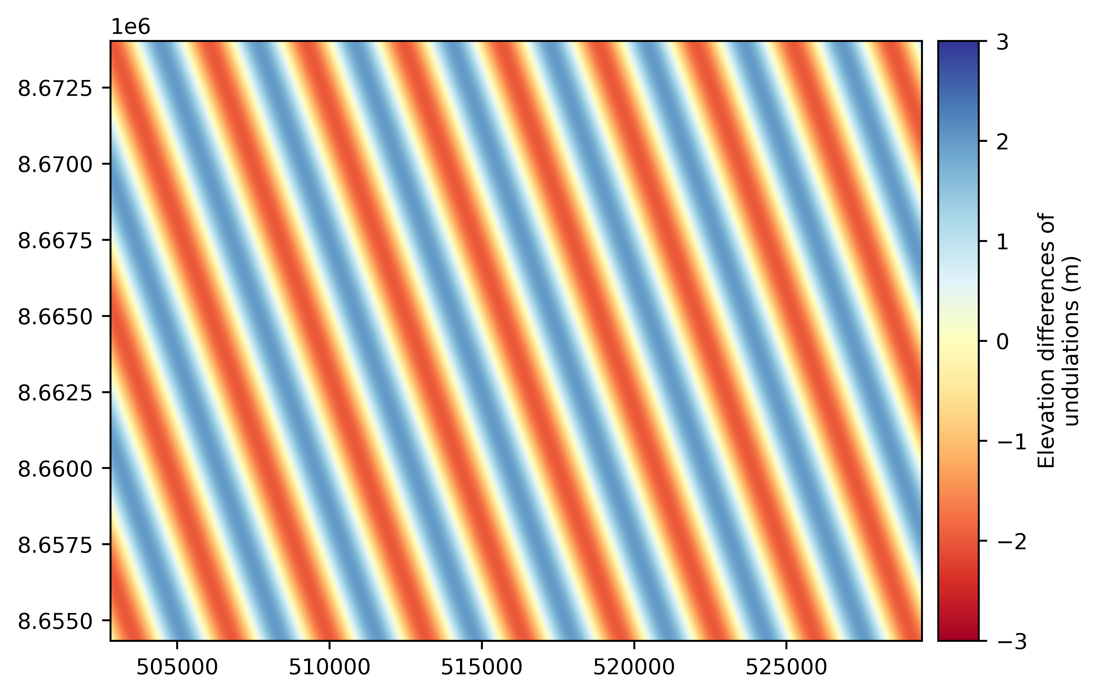
Undulations#
Example of undulations resembling jitter errors. We here artificially create a sinusoidal signal at a certain angle.
Point alternating#
An example of alternating point errors created by wrong point-raster comparison by rasterization of the points, which are especially large around steep slopes.
/home/docs/checkouts/readthedocs.org/user_builds/xdem/conda/stable/lib/python3.14/site-packages/geoutils/raster/raster.py:1822: UserWarning: Setting default nodata -99999 to mask non-finite values found in the array, as no nodata value was defined.
  warnings.warn(