Gap-filling#
xDEM contains routines to gap-fill elevation data or elevation differences depending on the type of terrain.
Important
Most of the approaches below are application-specific (e.g., glaciers) and might be moved to a separate package in future releases.
So far, xDEM has three types of gap-filling methods:
Inverse-distance weighting interpolation,
Local hypsometric interpolation (only relevant for elevation differences and glacier applications),
Regional hypsometric interpolation (also for glaciers).
The last two methods are described in McNabb et al. (2019).
We create a difference of DEMs object xdem.ddem.dDEM to experiment on:
ddem = xdem.dDEM(raster=dem_2009 - dem_1990, start_time=datetime(1990, 8, 1), end_time=datetime(2009, 8, 1))

# The example DEMs are void-free, so let's make some random voids.
# Introduce a fifth of nans randomly throughout the dDEM.
mask = np.zeros_like(ddem.data, dtype=bool)
mask.ravel()[(np.random.choice(ddem.data.size, int(ddem.data.size/5), replace=False))] = True
ddem.set_mask(mask)
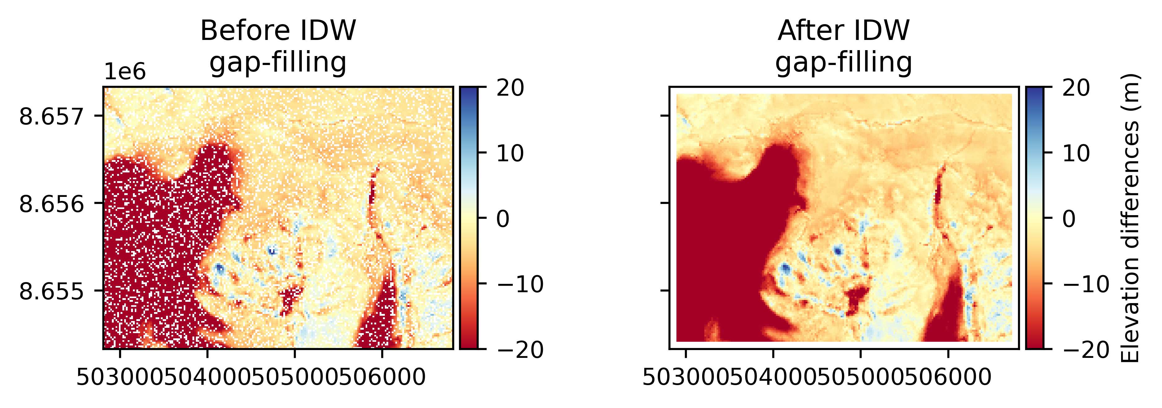
Inverse-distance weighting interpolation#
Inverse-distance weighting (IDW) interpolation of elevation differences is arguably the simplest approach: voids are filled by a weighted-mean of the surrounding pixels values, with weight inversely proportional to their distance to the void pixel.
ddem_idw = ddem.interpolate(method="idw")
/home/docs/checkouts/readthedocs.org/user_builds/xdem/conda/stable/lib/python3.14/site-packages/geoutils/raster/raster.py:1822: UserWarning: Setting default nodata -99999 to mask non-finite values found in the array, as no nodata value was defined.
  warnings.warn(
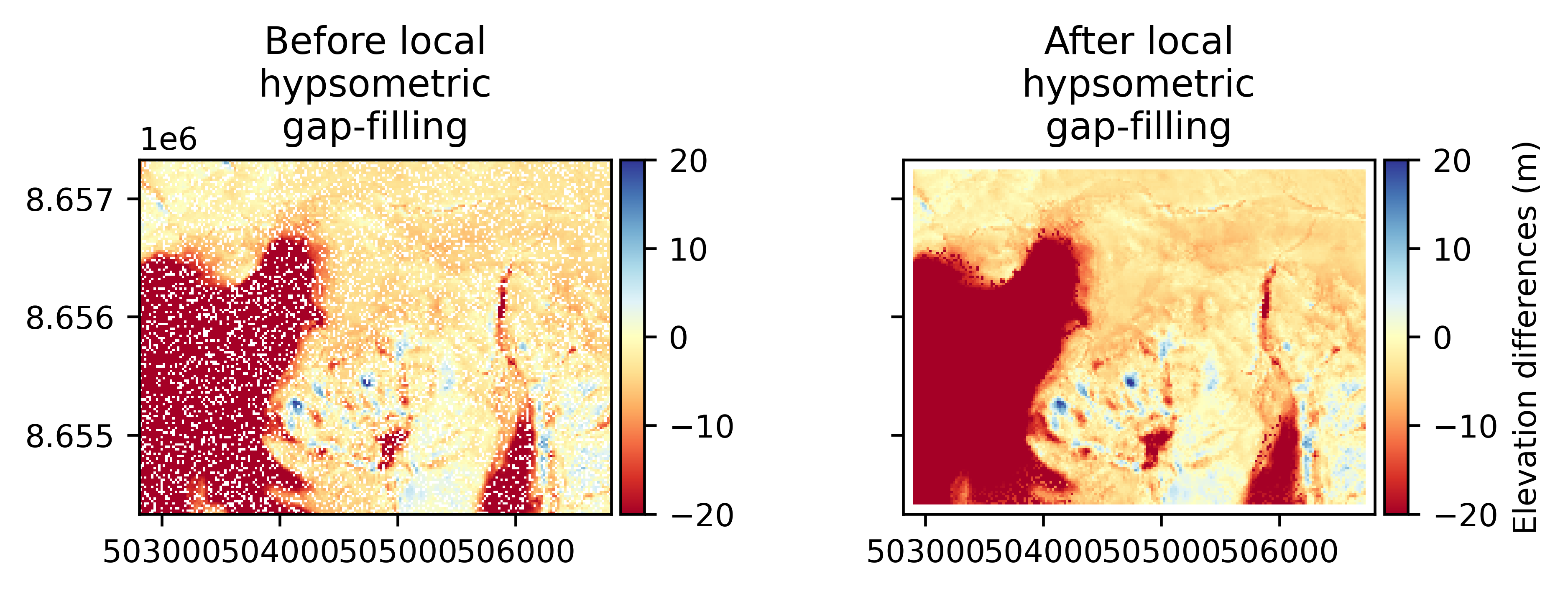
Local hypsometric interpolation#
This approach assumes that there is a relationship between the elevation and the elevation change in the dDEM, which is often the case for glaciers. Elevation change gradients in late 1900s and 2000s on glaciers often have the signature of large thinning in the lower parts, while the upper parts might be less negative, or even positive. This relationship is strongly correlated for a specific glacier, and weakly correlated on regional scales. With the local (glacier specific) hypsometric approach, elevation change gradients are estimated for each glacier separately. This is simply a linear or polynomial model estimated with the dDEM and a reference DEM. Then, voids are interpolated by replacing them with what “should be there” at that elevation, according to the model.
ddem_localhyps = ddem.interpolate(method="local_hypsometric", reference_elevation=dem_2009, mask=glaciers_1990)
/home/docs/checkouts/readthedocs.org/user_builds/xdem/conda/stable/lib/python3.14/site-packages/geoutils/raster/raster.py:1822: UserWarning: Setting default nodata -99999 to mask non-finite values found in the array, as no nodata value was defined.
  warnings.warn(
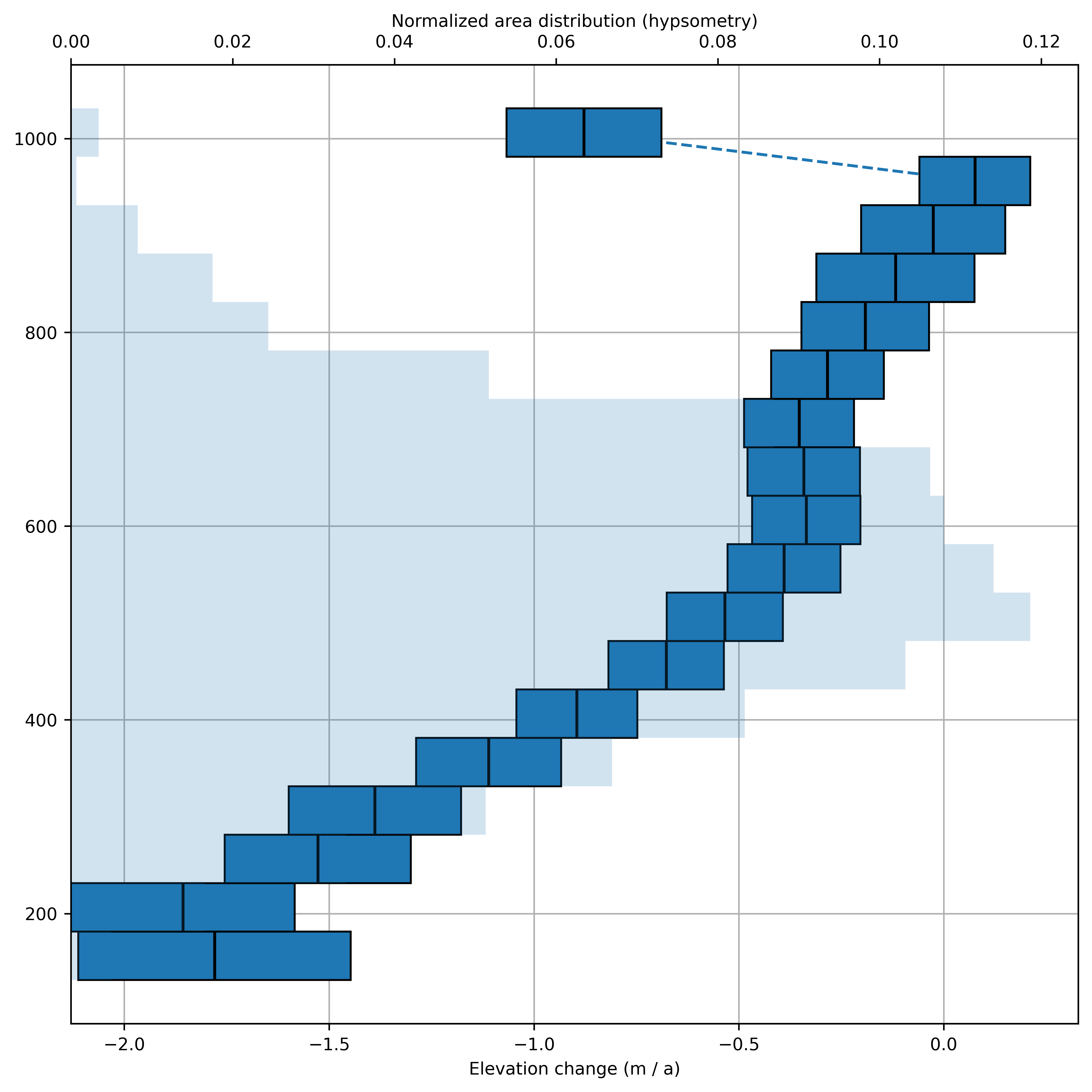
Where the binning can be visualized as such:
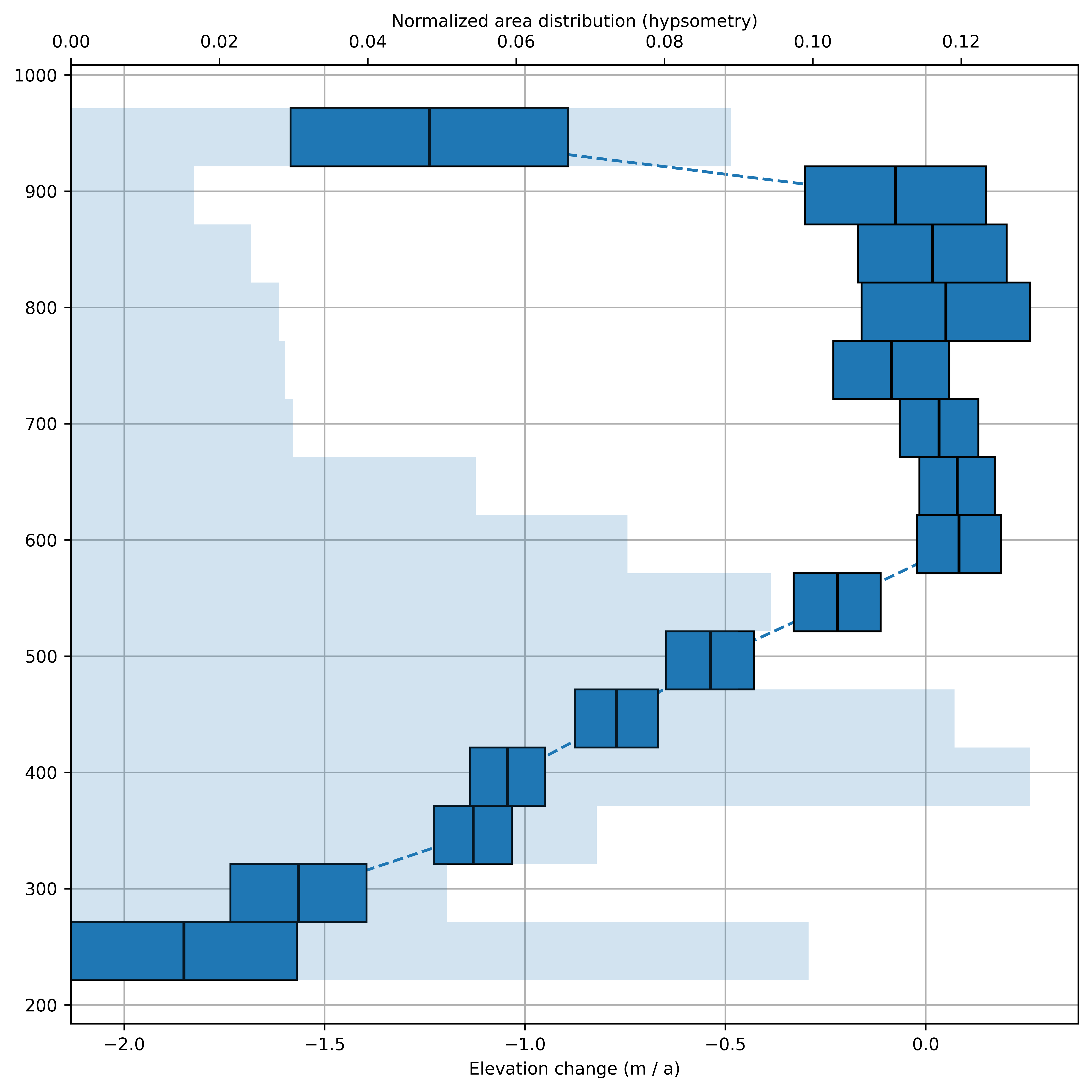
Caption: Hypsometric elevation change of Scott Turnerbreen on Svalbard from 1990–2009. The width of the bars indicate the standard deviation of the bin. The light blue background bars show the area distribution with elevation.
Regional hypsometric interpolation#
Similarly to local hypsometric interpolation, the elevation change is assumed to be largely elevation-dependent. With the regional approach (often also called “global”), elevation change gradients are estimated for all glaciers in an entire region, instead of estimating one by one.
ddem.set_mask(mask)
ddem_reghyps = ddem.interpolate(method="regional_hypsometric", reference_elevation=dem_2009, mask=glaciers_1990)
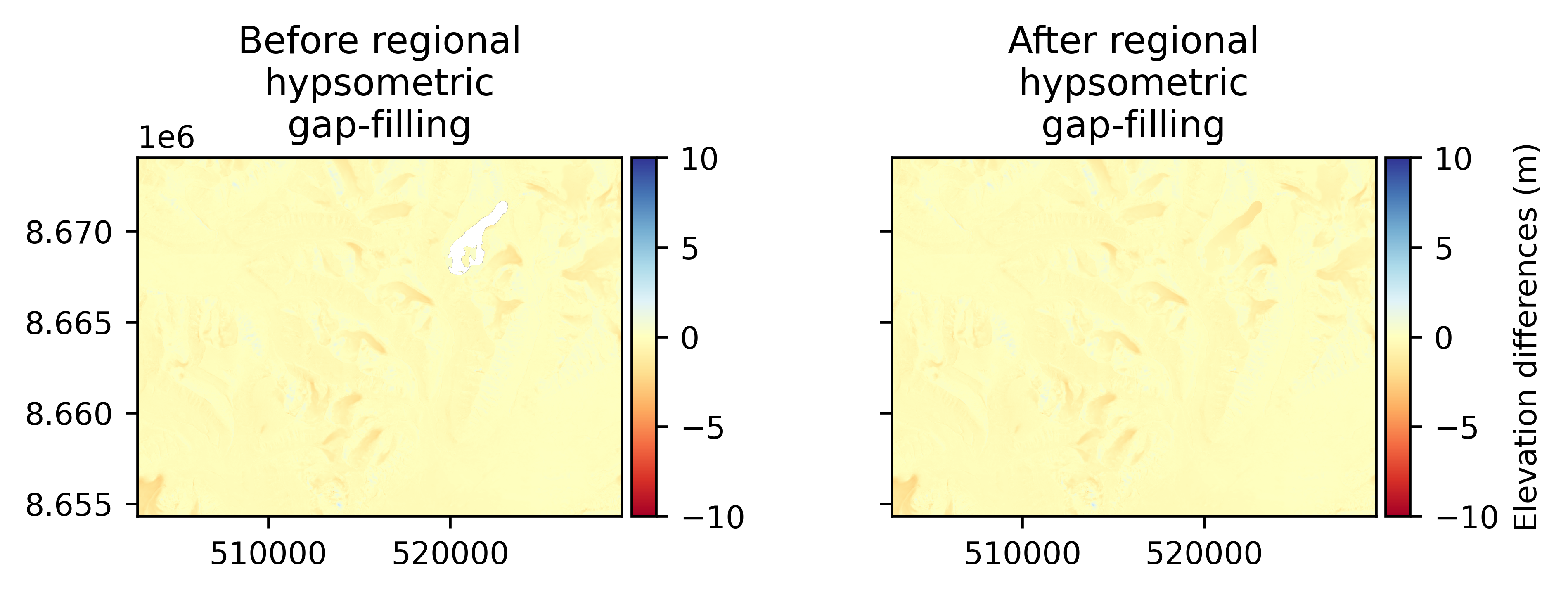
Caption: Regional hypsometric elevation change in central Svalbard from 1990–2009. The width of the bars indicate the standard deviation of the bin. The light blue background bars show the area distribution with elevation.