Spatial statistics for error analysis#
Performing error (or uncertainty) analysis of spatial variable, such as elevation data, requires joint knowledge from two scientific fields: spatial statistics and uncertainty quantification.
Spatial statistics, also referred to as geostatistics in geoscience, is a body of theory for the analysis of spatial variables. It primarily relies on modelling the dependency of variables in space (spatial autocorrelation) to better describe their spatial characteristics, and utilize this in further quantitative analysis.
Uncertainty quantification is the science of characterizing uncertainties quantitatively, and includes a wide range of methods including in particular theoretical error propagation. In measurement science, such as remote sensing, such uncertainty propagation is tightly linked with the field of metrology.
In the following, we describe the basics assumptions and concepts required to perform a spatial uncertainty analysis of elevation data, described in the feature page Uncertainty analysis.
Assumptions for inference in spatial statistics#
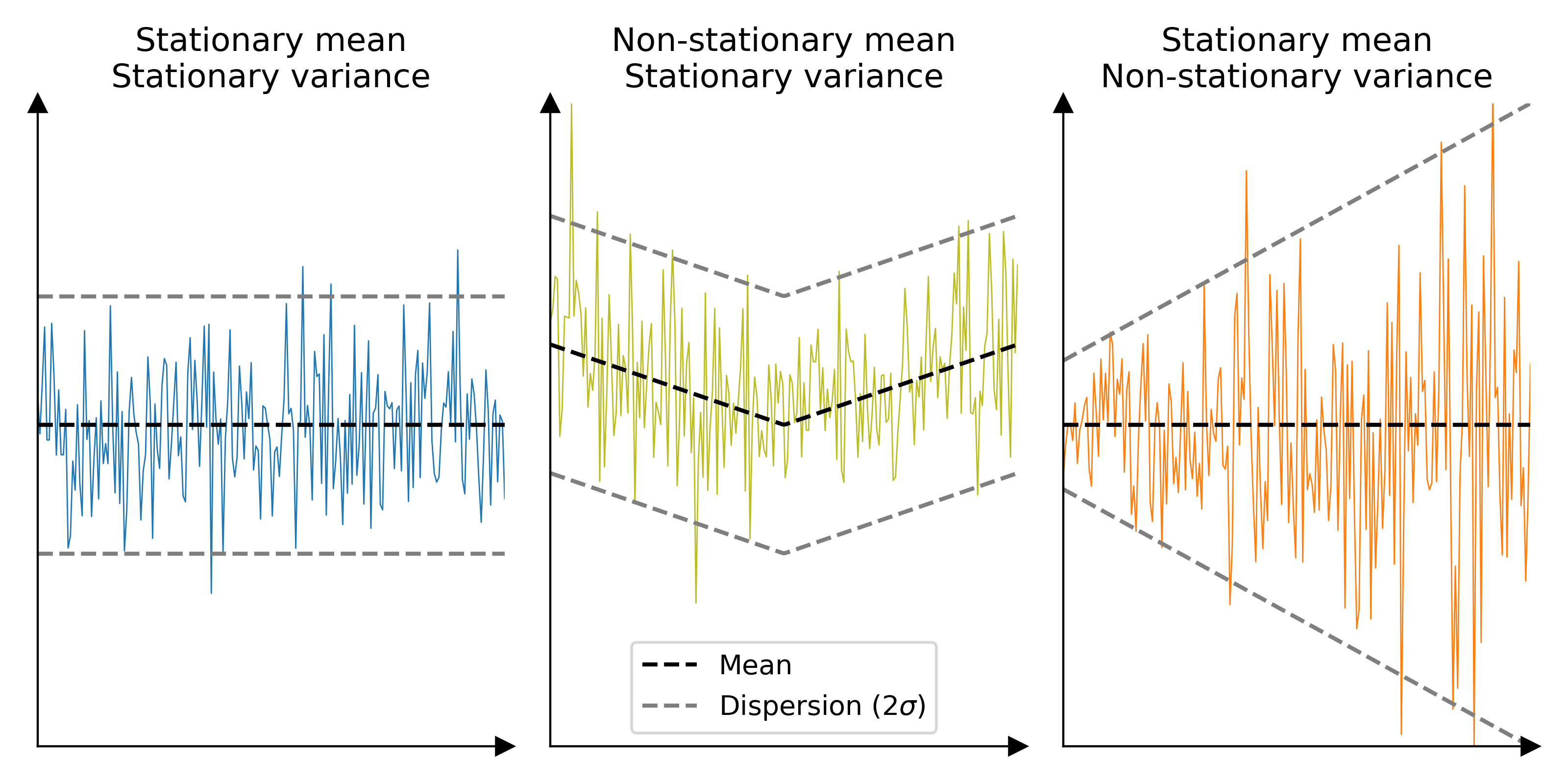
In spatial statistics, the covariance of a variable of interest is generally simplified into a spatial variogram, which describes the covariance only as function of the spatial lag (spatial distance between two variable values). However, to utilize this simplification of the covariance in subsequent analysis, the variable of interest must respect the assumption of second-order stationarity. That is, verify the three following assumptions:
The mean of the variable of interest is stationary in space, i.e. constant over sufficiently large areas,
The variance of the variable of interest is stationary in space, i.e. constant over sufficiently large areas.
The covariance between two observations only depends on the spatial distance between them, i.e. no other factor than this distance plays a role in the spatial correlation of measurement errors.
(Source code, .png)
In other words, for a reliable analysis, elevation data should:
Not contain elevation biases that do not average out over sufficiently large distances (e.g., shifts, tilts), but can contain pseudo-periodic biases (e.g., along-track undulations),
Not contain random elevation errors that vary significantly across space.
Not contain factors that affect the spatial distribution of elevation errors, except for the distance between observations.
While assumption 1. is verified after coregistration and bias corrections, other assumptions are generally not (e.g., larger errors on steep slope). To address this, we must estimate the variability of our random errors (or heteroscedasticity), to then transform our data to achieve second-order stationarity.
Note
If there is no significant spatial variability in random errors in your elevation data (e.g., lidar), you can jump directly to the Spatial correlation of errors section.
Heteroscedasticity#
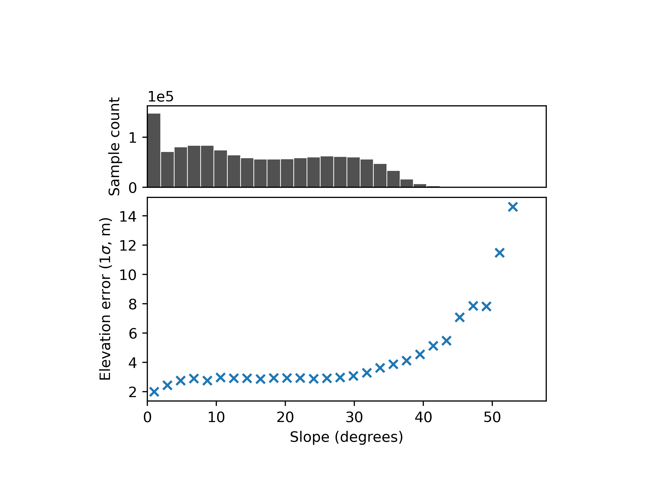
Elevation heteroscedasticity corresponds to a variability in precision of elevation observations, that are linked to terrain or instrument variables.
While a single elevation difference (for a pixel or footpring) does not allow to capture random errors, larger samples do. Data binning, for instance, is a method that allows to estimate the statistical spread of a sample per category, and can easily be used with one or more explanatory variables, such as slope:
(Source code, .png)

Then, a model (parametric or not) can be fit to infer the variability of random errors at any data location.
Standardization#
In order to verify the assumptions of spatial statistics and be able to use stable terrain as a reliable proxy in further analysis (see Static surfaces as error proxy guide page), standardization of the elevation differences by their mean \(\mu\) and spread \(\sigma\) are required to reach a stationary variance.
(Source code, .png)
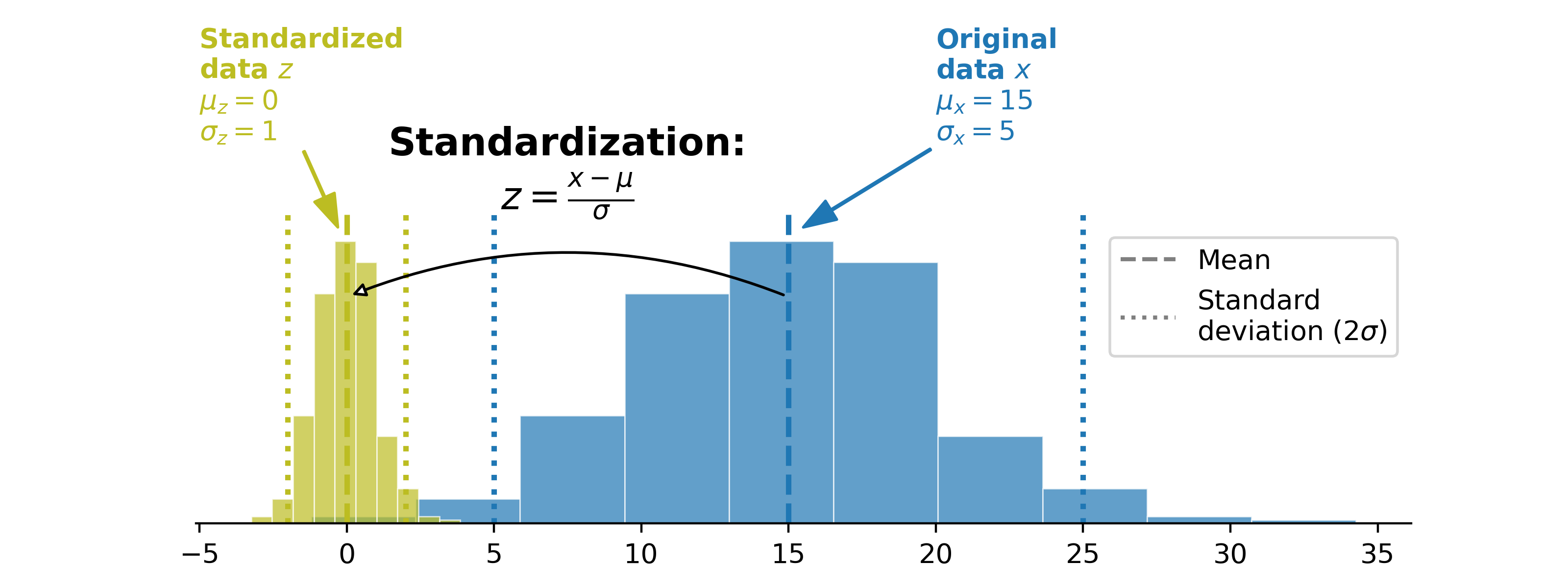
For elevation differences, the mean is already centered on zero but the variance is non-stationary, which yields more simply:
where \(z_{dh}\) is the standardized elevation difference sample.
Spatial correlation of errors#
Spatial correlation of elevation errors correspond to a dependency between measurement errors of spatially close pixels in elevation data. Those can be related to the resolution of the data (short-range correlation), or to instrument noise and deformations (mid- to long-range correlations).
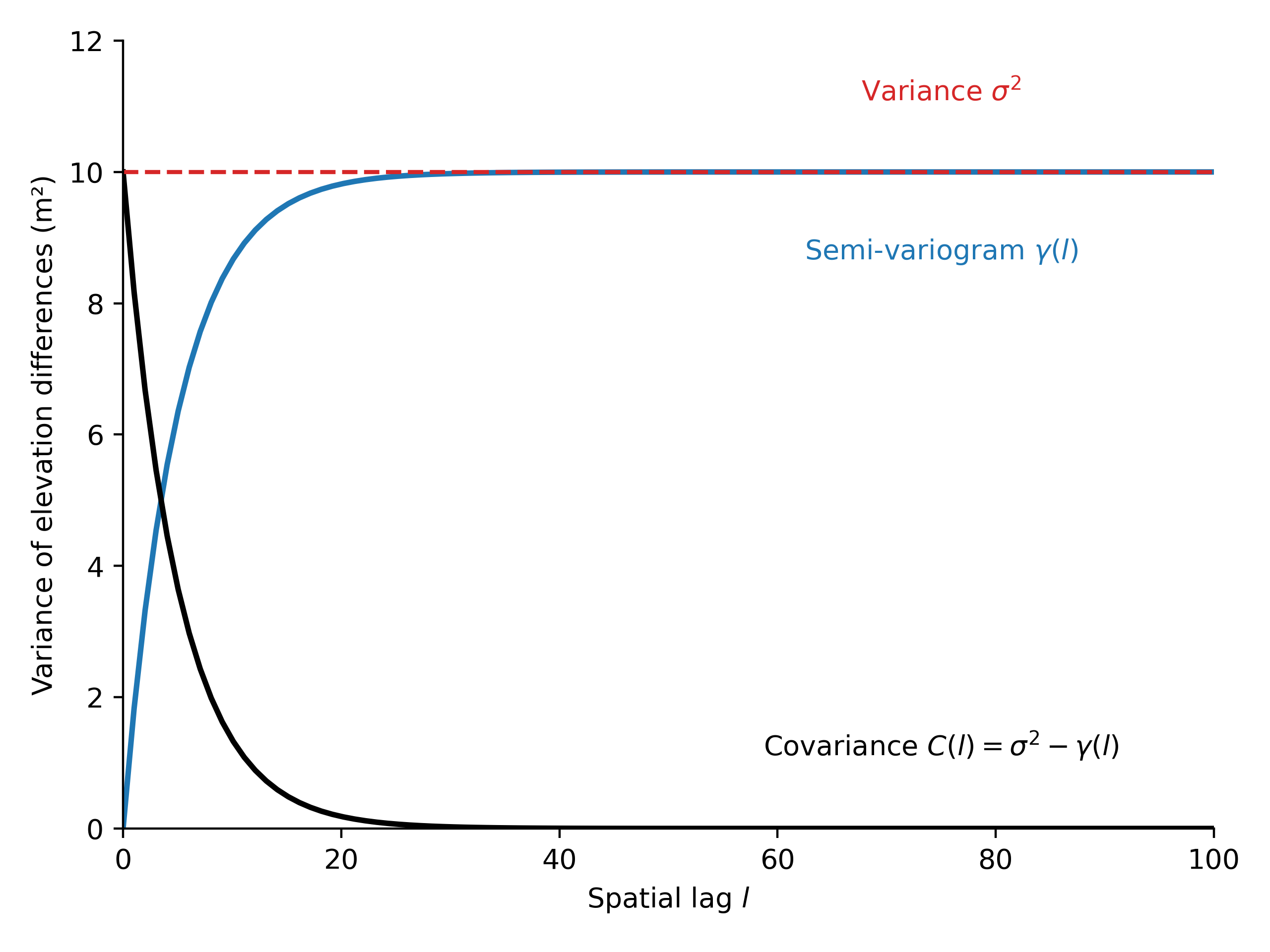
Variograms are functions that describe the spatial correlation of a sample. The variogram \(2\gamma(h)\) is a function of the distance between two points, referred to as spatial lag \(d\). The output of a variogram is the correlated variance of the sample.
where \(Z(\textrm{s}_{i})\) is the value taken by the sample at location \(\textrm{s}_{i}\), and sample positions \(\textrm{s}_{1}\) and \(\textrm{s}_{2}\) are separated by a distance \(d\).
(Source code, .png)
For elevation differences \(dh\), this translates into:
The variogram essentially describes the spatial covariance \(C\) in relation to the variance of the entire sample \(\sigma_{dh}^{2}\):
Variograms are estimated empirically by data binning depending on the pairwise distance among data points, then modelled by functional forms called variogram models (e.g., spherical, gaussian).
As pairwise combinations grow exponentially with data points, variograms are estimated using a random subsample of the elevation data (whether gridded or point). Additionally, as elevation data usually contains patterns of correlation at both short-range (close to pixel size) and long-range (close to DEM extent), the default pairwise sampling can be tuned to perform well at all desired ranges.
Note
In xDEM, variograms use by default a subsample size of 1000 data points (leading to 500,000 pairwise differences estimated), for computational efficiency. xDEM also uses by default a random sampling method that selects a uniform amount of data points by pairwise log-distance, in order to capture potential correlations at all ranges.
For more details on variography, we refer to the documentation of SciKit-GStat.
Error propagation#
Once the heteroscedasticity \(\sigma_{dh}(\textrm{var}_{1},\textrm{var}_{2}, \textrm{...})\) and spatial correlation of errors \(\gamma_{dh}(d)\) are both estimated, those can be used to propagate errors to derivatives of the elevation data.
For simple derivatives such as spatial derivatives (e.g., mean or sum in an area), exact theoretical propagation relying on the above components can be employed.
For instance, to propagate errors to the mean of elevation differences in an area \(A\) containing \(N\) data points:
where \(d_{ij}\) is the distance between data point \(i\) and \(j\).
Note
xDEM implement several methods to approximate the above equation which scales exponentially with data points, to preserve computational efficiency.
For more complex derivatives such as terrain attributes, the heteroscedasticity and spatial correlation of errors can be used to constrain simulation methods that numerically generate realizations of the structure of errors.
For instance, to propagate errors to terrain slope, one can derive many realizations of random fields based on the error structure estimated for the DEM. Then, for each realization, add the random field to the DEM, and derive its slope. Finally, the error in slope can be estimated from the spread of all slope realizations.
References and more reading
For random field generation, see for example GSTools.
References:
Heuvelink et al. (1989), Propagation of errors in spatial modelling with GIS,
Rolstad et al. (2009), Spatially integrated geodetic glacier mass balance and its uncertainty based on geostatistical analysis: Application to the western Svartisen ice cap, Norway,
Hugonnet et al. (2022), Uncertainty analysis of digital elevation models by spatial inference from stable terrain.